引言

在数据库查询优化器中，Join Reordering（连接重排） 是一项至关重要的优化技术。在涉及多个表的复杂连接查询中，不同的连接顺序可能导致执行效率相差数个数量级。然而，可能的连接顺序数量随表的数量呈阶乘级增长，使得在一般情况下，寻找最优连接顺序成为一个 NP-hard 问题。Join Reordering 优化的核心目标，正是在庞大的搜索空间中高效地探索并选择一个接近最优（或可接受）的连接顺序，以显著提升查询性能。

在DuckDB中，有两个优化是和Join Reorder相关的：JOIN_ORDER和BUILD_SIDE_PROBE_SIDE。我们先来说一下这两个优化的作用，JOIN_ORDER优化负责对多个表的Join的顺序进行优化，例如对于三个表， 该优化会在，，中寻找最优的Join Order，有读者可能发现，JOIN_ORDER优化可能有些Join顺序没有枚举到，这是因为在这个优化中，由于代价计算只考虑参与Join的表的基数和结果集的基数，这也就导致和的代价是完全相同的，但我们知道对于Hash Join，使用小表构建哈希表，使用大表作为探测表，性能通常是更优的，因此在BUILD_SIDE_PROBE_SIDE优化中，就负责对参与Hash Join的两个表依据哈希表的大小进行交换，比如我们在JOIN_ORDER优化中，确认是最优的Join Order，那么在BUILD_SIDE_PROBE_SIDE中，就会去尝试交换和以及和。

我们先通过一个例子看一下DuckDB的Join Reorder算法的性能，假设我们有如下表结构：

CREATE TABLE t1 (    id int,    col1 int,    col2 int,    col3 int,    col4 int,    col5 int,    col6 int);CREATE TABLE t2 AS FROM t1;CREATE TABLE t3 AS FROM t1;CREATE TABLE t4 AS FROM t1;CREATE TABLE t5 AS FROM t1;CREATE TABLE t6 AS FROM t1;

现在考虑如果我们有这样一条SQL，我们要如何去枚举它的Join Order：

SELECT t1.idFROM t1, t2, t3, t4, t5, t6WHERE t1.col1 = t2.col1    AND t2.col2 = t3.col2    AND t4.col4 = t5.col4    AND t5.col5 = t6.col5    AND t1.id + t2.id + t3.id = t4.id + t5.id + t6.id;

在MySQL中，由于只会枚举Left Deep Tree的JOIN ORDER，在表中无任何数据的情况，会得到如下执行计划：

-> Filter: (((t1.id + t2.id) + t3.id) = ((t4.id + t5.id) + t6.id))  (cost=2.1 rows=1)    -> Inner hash join (t6.col5 = t5.col5)  (cost=2.1 rows=1)        -> Table scan on t6  (cost=0.35 rows=1)        -> Hash            -> Inner hash join (t5.col4 = t4.col4)  (cost=1.75 rows=1)                -> Table scan on t5  (cost=0.35 rows=1)                -> Hash                    -> Inner hash join (no condition)  (cost=1.4 rows=1)                        -> Table scan on t4  (cost=0.35 rows=1)                        -> Hash                            -> Inner hash join (t3.col2 = t2.col2)  (cost=1.05 rows=1)                                -> Table scan on t3  (cost=0.35 rows=1)                                -> Hash                                    -> Inner hash join (t2.col1 = t1.col1)  (cost=0.7 rows=1)                                        -> Table scan on t2  (cost=0.35 rows=1)                                        -> Hash                                            -> Table scan on t1  (cost=0.35 rows=1)

在该执行计划中，t1到t6按照顺序进行Join，在Join t4表的时候，由于没有Join Condition，因此会进行笛卡尔积，最后通过一个Filter过滤满足t1.id + t2.id + t3.id = t4.id + t5.id + t6.id满足的数据。

这样的Join Order明显不是最优的，我们可以先将t1表到t3表进行Join，再将t4表到t6表进行Join，最后利用t1.id + t2.id + t3.id = t4.id + t5.id + t6.id将上述两次Join的结果集进行Hash Join。

我们来看下DuckDB生成的执行计划：

┌─────────────────────────────┐│┌───────────────────────────┐│││       Physical Plan       │││└───────────────────────────┘│└─────────────────────────────┘┌───────────────────────────┐│         PROJECTION        ││    ────────────────────   ││             #0            ││                           ││           ~1 row          │└─────────────┬─────────────┘┌─────────────┴─────────────┐│         HASH_JOIN         ││    ────────────────────   ││      Join Type: INNER     ││                           ││        Conditions:        ├────────────────────────────────────────────────────────────────────────┐│ ((id + id) + id) = ((id + │                                                                        ││          id) + id)        │                                                                        ││                           │                                                                        ││           ~1 row          │                                                                        │└─────────────┬─────────────┘                                                                        │┌─────────────┴─────────────┐                                                          ┌─────────────┴─────────────┐│         HASH_JOIN         │                                                          │         HASH_JOIN         ││    ────────────────────   │                                                          │    ────────────────────   ││      Join Type: INNER     │                                                          │      Join Type: INNER     ││                           │                                                          │                           ││        Conditions:        ├───────────────────────────────────────────┐              │        Conditions:        ├───────────────────────────────────────────┐│        col1 = col1        │                                           │              │        col4 = col4        │                                           ││                           │                                           │              │                           │                                           ││           ~1 row          │                                           │              │           ~1 row          │                                           │└─────────────┬─────────────┘                                           │              └─────────────┬─────────────┘                                           │┌─────────────┴─────────────┐                             ┌─────────────┴─────────────┐┌─────────────┴─────────────┐                             ┌─────────────┴─────────────┐│         HASH_JOIN         │                             │         SEQ_SCAN          ││         HASH_JOIN         │                             │         SEQ_SCAN          ││    ────────────────────   │                             │    ────────────────────   ││    ────────────────────   │                             │    ────────────────────   ││      Join Type: INNER     │                             │         Table: t1         ││      Join Type: INNER     │                             │         Table: t4         ││                           │                             │   Type: Sequential Scan   ││                           │                             │   Type: Sequential Scan   ││        Conditions:        │                             │                           ││        Conditions:        │                             │                           ││        col2 = col2        ├──────────────┐              │        Projections:       ││        col5 = col5        ├──────────────┐              │        Projections:       ││                           │              │              │            col1           ││                           │              │              │            col4           ││                           │              │              │             id            ││                           │              │              │             id            ││                           │              │              │                           ││                           │              │              │                           ││           ~1 row          │              │              │          ~0 rows          ││           ~1 row          │              │              │          ~0 rows          │└─────────────┬─────────────┘              │              └───────────────────────────┘└─────────────┬─────────────┘              │              └───────────────────────────┘┌─────────────┴─────────────┐┌─────────────┴─────────────┐                             ┌─────────────┴─────────────┐┌─────────────┴─────────────┐│         SEQ_SCAN          ││         SEQ_SCAN          │                             │         SEQ_SCAN          ││         SEQ_SCAN          ││    ────────────────────   ││    ────────────────────   │                             │    ────────────────────   ││    ────────────────────   ││         Table: t2         ││         Table: t3         │                             │         Table: t5         ││         Table: t6         ││   Type: Sequential Scan   ││   Type: Sequential Scan   │                             │   Type: Sequential Scan   ││   Type: Sequential Scan   ││                           ││                           │                             │                           ││                           ││        Projections:       ││        Projections:       │                             │        Projections:       ││        Projections:       ││            col1           ││            col2           │                             │            col4           ││            col5           ││            col2           ││             id            │                             │            col5           ││             id            ││             id            ││                           │                             │             id            ││                           ││                           ││                           │                             │                           ││                           ││          ~0 rows          ││          ~0 rows          │                             │          ~0 rows          ││          ~0 rows          │└───────────────────────────┘└───────────────────────────┘                             └───────────────────────────┘└───────────────────────────┘

可以看到DuckDB生成的Join Order与我们的预期是相符的。

那么对于MySQL而言，可能生成这种执行计划么？MySQL默认情况下的Join Reorder算法只能去枚举Left Deep Tree的Join Order，而这种Join Order是Bushy Tree，因此无论表中数据如何，MySQL都无法生成这种执行计划。不过，MySQL中有一个参数hypergraph_optimizer，当该参数开启时，就可以去枚举这种Bushy Tree的Join Order，从而得到这种执行计划。

其实DuckDB和MySQL的hypergraph_optimizer都使用了同一种Join Order枚举算法DpHyp，DpHyp算法也是JOIN_ORDER优化中的核心算法，该算法比较复杂，在本文，我们将首先介绍DpHyp算法，再结合DuckDB源码来看JOIN_ORDER优化和BUILD_SIDE_AND_PROBE_SIDE算法。

Dphyp算法

Dphyp算法，出自论文《Dynamic Programming Strikes Back》，从字面理解，就是Dynamic Programming和HyperGraph。那么我们首先就要搞清楚，Dynamic Programming是如何应用于Join Order的求解的。

Dynamic Programming是如何应用于Join Order的求解的原理其实很简单，就是当求解n个表Join时，这个问题可以转换为求解1个表和n-1表进行Join，从而就出现了子问题，可以使用DP算法求解。

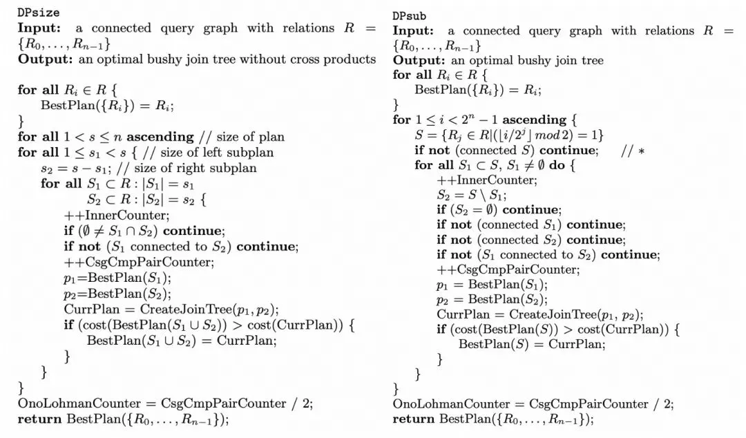
DPsize算法和DPsub算法是使用Dynamic Programming求解Join Order的经典算法，它们二者唯一的区别就是在枚举顺序上，Dpsize算法不断增加参与Join的表的个数，而Dpsub算法按照bitmap的方式进行枚举，例如，四个表t1，t2，t3，t4进行join，Dpsize算法会按照两个表Join，三个表Join，四个表Join进行枚举，而Dpsub算法将表编码为四个bit的二进制数，二进制数1010就代表t4和t2表进行Join，按照0001，0010，0011，0100，0101，…的顺序依次枚举。

但使用这种简单Dp算法，我们可能会枚举到很多无意义的Join Order，例如，我们有SQL：SELECT * FROM t1 JOIN t2 ON t1.col1 = t2.col1 JOIN t3 ON t2.col2 = t3.col2;，那么DPsize算法会按照({t1}, {t2})，({t2}, {t1})，({t1},{t3})，({t3}, {t1})，({t2}, {t3})，({t3},{t2})，({t1}, {t2,t3})，({t2}, {t1,t3})，({t3}, {t1,t2})，({t1,t2}, {t3})，({t1,t3}, {t2})，({t2,t3}, {t1})的顺序枚举。但其实例如({t1},{t3})，({t3}, {t1})，({t2}, {t1,t3})等Join Order没必要计算，因为t1和t3之间根本没有可供连接的谓词，造成这个现象的原因是我们枚举Join Order没有考虑连接关系。

而Dphyp算法将SQL的连接关系转换为超图，从而能够更有效地进行Join Order枚举，本文我们就重点讲解Dphyp算法，并且结合DuckDB源码进行说明，我们首先结合引言中的SQL来看一下DpHyp中基本定义。

HyperGraph（超图）

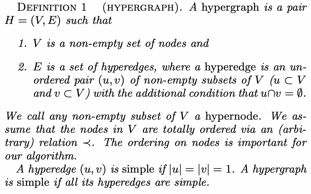
超图H=(V,E)由节点集合V和超边集合E构成，其中超边的两个超节点u,v是节点集合V的子集，并且u和v没有交集。

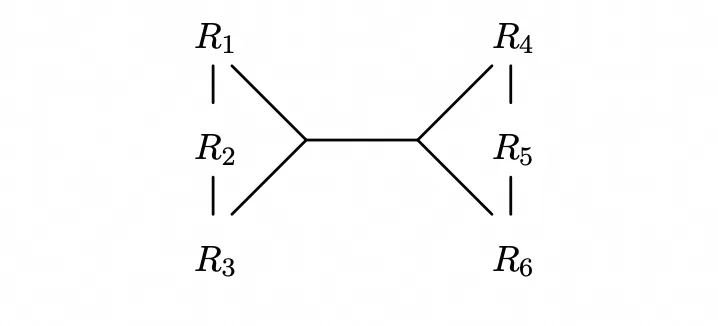
在有了这个定义后，对于一条SQL，每个表其实都是一个节点，每个连接关系都是超边。以上述SQL为例，我们就获得了超图$$$$

其中我们还需要节点之间存在一个顺序关系，这个顺序关系是可以任意指定的，但必须存在，因为这个会影响算法对于Join Order的枚举顺序，在这个SQL中，可以直接按照表名来进行排序。

SubGraph（子图）

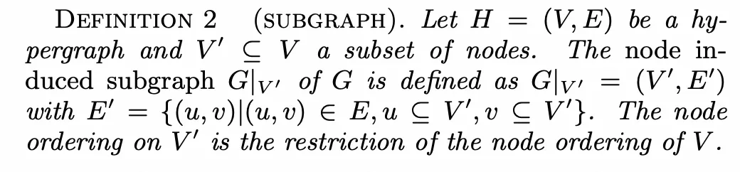
对于超图，节点集合V的一个子集可以诱导出一个子图，记做，其中是的一个子集，并且中所有超边的两个端点都必须是的子集。

还是以上述SQL为例，如果，那么它的诱导出的子图的超边集合为。

Connected（连通性）

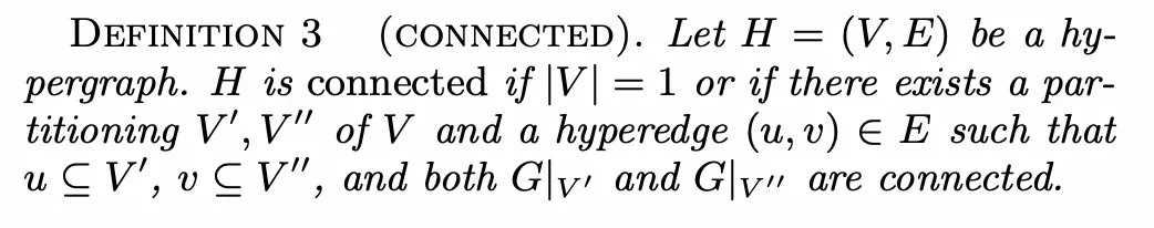
如果一个超图中只有一个节点，那么这个超图是连通的。

如果一个超图有大于两个节点，那么只要存在一种划分和一条属于的超边，使得超边的两端集合分别属于，并且分别诱导出的子图也是联通的，则这个超图是连通的。

上述SQL所构造出的超图就是连通的，因为我们可以将其划分为，两个节点集合可以由相连，并且各自诱导出的子图也是连通的。

需要注意的是，不一定所有的SQL表示成的超图都是连通的，但总可以在不连通的连通分量之间添加一条表示笛卡尔积的超边使得整个超图连通，且添加前后不影响SQL的结果。

Csg-cmp-pair（连通子图-连通补图-对）

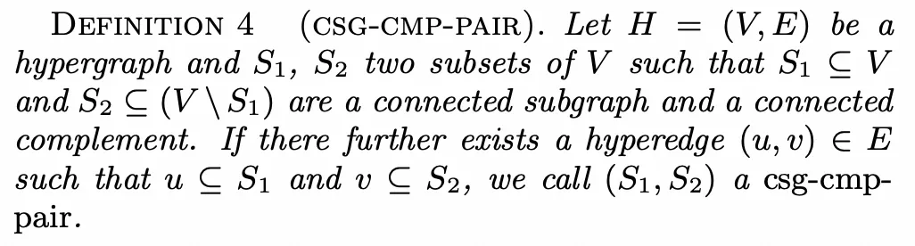
对于超图，节点集合V的子集诱导出的子图是连通的，那么我们称为连通子图（严格来说是只是节点集合，不是图，此处是为了方便直接称它为连接子图）,简称csg。如果节点集合是在中补集的子集，并且它诱导出的子图也是连通的，我们称是的连通补图，简称cmp。如果和能有一条超边将其连接，我们称是连通子图-连通补图-对，简称csg-cmp-pair。

还是以上述SQL为例，和就是csg-cmp-pair，但和就不是。

显然，我们使用动态规划算法枚举Join Order，其实就是在枚举所有的csg-cmp-pair的，例如，对于找到csg-cmp-pair：和，其实就代表了t1，t2，t3先join，t4，t5，t6表再join，两次join的结果集再进行join。为了符合动态规划的要求，csg-cmp-pair的枚举也是有顺序要求的，而Dphyp算法的核心也就是解决枚举顺序。

Neighborhood（邻居节点）

对于一个简单图，邻居节点很好定义，但对于一个超图中超边的存在，邻居节点的定义就发生了变化。

超图的中的邻居是针对节点集的而不是节点，因此我们需要评估的是例如这种节点集在超图中的邻居。一个很直观的定义是，假设存在一条超边，超边的一个超节点是的子集，另一个超节点与不相交，那么我们可以将作为的邻居，用公式表示如下：

但对于我们枚举csg-cmp-pair而言，这个定义还可以优化：对于v中所有节点，并不需要全部列为邻居，因为它们在S_1看来是完全等价的，我们只需要选取其中一个即可。

因此我们对邻居的定义进行优化：

其中代表了超节点中排序关系最小的节点，例如对于，有。

这个定义还可以优化，假设存在两条超边，超边的超节点存在关系，那么其实只需要考虑中节点。例如，如果我们在图中还存在一条超边，那么对于的邻居并不需要定义为，只需要定义为即可，在论文中，使用表示进行过这种优化的超节点集合。此时邻居的定义就为：

最后，我们对邻居的定义再附加一个参数X，要求超节点，这个定义是用来保证枚举顺序的，最终就构成我们对于邻居节点的定义。

算法流程

Dphyp算法是由五个子函数构成的，分别是Solve，EnumerateCsgRec，EmitCsg，EnumerateCmpRec，EmitCsgCmp函数。为了理解方便，在本文中使用与论文中不同的顺序介绍这五个函数。

EmitCsgCmp

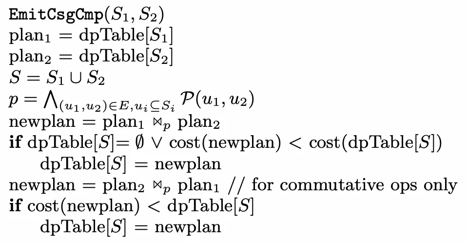
当我们成功找到了一个csg-cmp-pair时，会调用这个函数，这个函数负责在dpTable中记录这种Join Order的cost。其中是我们找到的csg-cmp-pair，p是进行Join所用predicate，求解 Join 和 Join 的cost（如果Join ops满足交换律），更新dpTable[S]。

EnumerateCmpRec

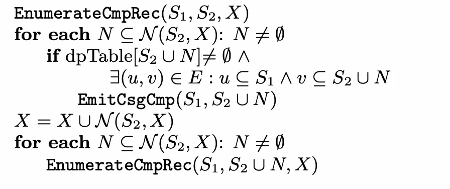
对于两个节点集合和，他们两个可能暂时无法构成csg-cmp-pair，因为不存在一条超边将他们相连，但却可以将按照连通性进行拓展，使得它们构成csg-cmp-pair，X是排除集，要求按照连通性拓展的节点不能在排除集之中，排除集的存在保证了找cmp时不会重复找到某个节点。

例如当时，，我们发现与之间不存在超边，因此再次调用EnumerateCmpRec函数，此时，，我们发现与之间存在超边，因此就构成了csg-cmp-pair，此时可以调用EmitCsgCmp函数去求解cost更新dpTable。

EmitCsg

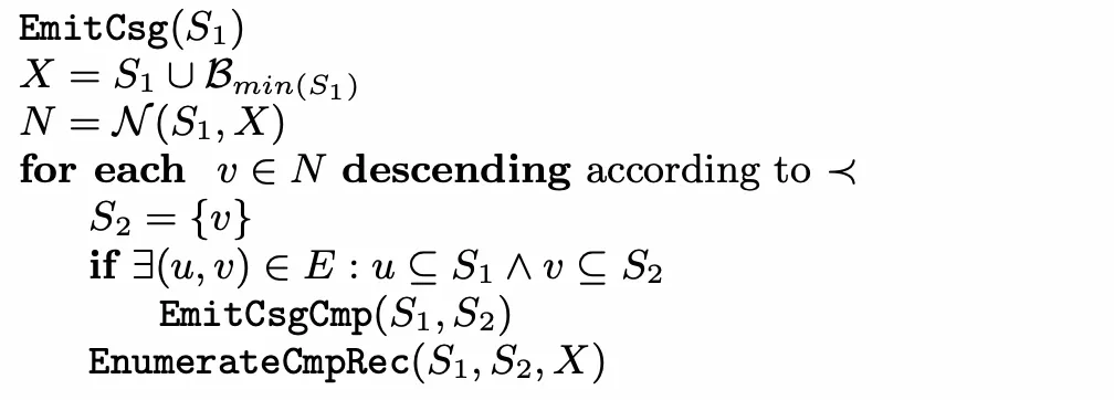
对于一个csg，我们需要考虑对这个csg找到它的cmp，而寻找csg就是从的邻居开始做拓展。

首先我们获取到排除集，排除集定义为，其中是所有排序关系小于等于节点的集合，例如，之所以要定义排除集，是因为我们需要枚举的顺序性，具体的原理解释我们留到Solve函数说明。

我们按照排序关系降序遍历的邻居，并且将初始化为这个邻居，如果和能直接构成csg-cmp-pair，那么调用EmitCsgCmp求解cost。最后调用EnumerateCmpRec，去考虑拓展。

EnumerateCsgRec

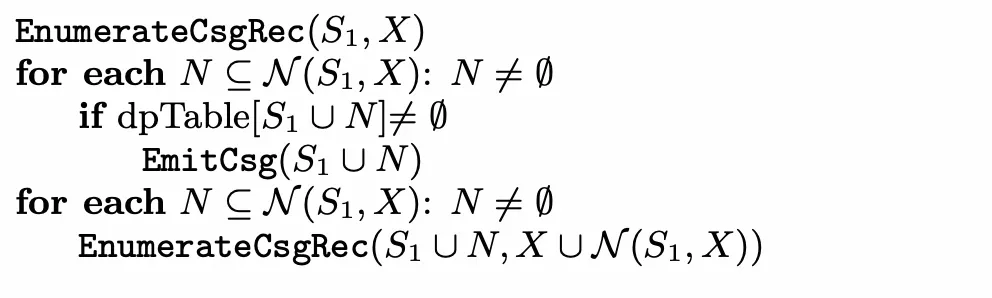
对于一个节点集合，我们需要尽可能拓展节点来枚举csg，因此，我们首先去dpTable中逐个判断它的邻居能够与它构成csg，如果能够构成，则调用EmitCsg去寻找这个csg的cmp。做完之后，递归地调用EnumerateCsgRec不断判断新的节点集合是否能够通过邻居拓展来构成csg。

Solve

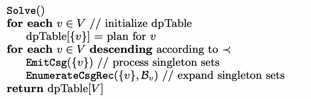
该函数是整个算法的入口函数，该函数首先初始化单个节点的dpTable，然后对于节点集合的每个节点，按照降序，首先调用EmitCsg函数来判断该节点能否与邻居节点构成csg-cmp-pair，然后从该节点出发，沿着邻居去拓展节点集合，判断当前子图是否连通。

这里需要注意，枚举v是降序枚举的，因此当枚举到时，我们就已经找到了所有节点间的csg和cmp，而对于的连通关系还不知道，因此在EmitCsg函数，我们定义了，这就是因为对于的cmp需要在中寻找，但此时中的连通关系还没确定，所以就只能在中寻找。

整个算法的流程还是比较清晰的，就是从单一节点出发，不断根据邻居关系拓展当前子图，如果当前子图的连通的，则代表找到了csg，然后在根据这个csg的邻居关系去找它的cmp，而找cmp的过程也可以再通过的邻居关系不断拓展，最终找到所有的csg-cmp-pair，保证枚举的正确性。而排他集能够保证枚举的顺序性。

但其实，论文中给出的算法流程存在缺陷，还是会导致重复枚举，我们来看一条简单的SQL：

SELECT *FROM t1, t2, t3WHERE t1.col1 = t2.col1    AND t2.col2 = t3.col2    AND t3.col3 = t1.col3;

SQL非常简单，三个表代表的节点互为邻居，当我们在solve函数中对枚举到t1时，此时，首先，调用时，会通过连通性拓展为，此时t1 JOIN (t2 JOIN t3)这个Join Order被枚举过了。当，调用时，会通过连通性拓展为，此时t1 JOIN (t2 JOIN t3)这个Join Order又被枚举一次。我们可以对算法伪代码进行些修改来避免这种重复枚举。修改后的EmitCsg函数如下：

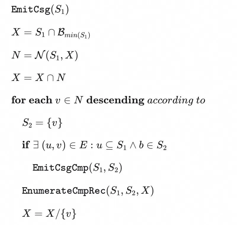
修改其实很简单，就是要保证如果S_1的邻居节点也是互为邻居的话，也需要根据顺序关系去拓展Cmp，应用到上面的例子：

，X会首先被拓展为，首先，调用时，就不会通过连通性拓展为，此时t1 JOIN (t2 JOIN t3)这个Join Order不会被枚举。之后X会取差集变成，调用时，通过连通性拓展为，此时t1 JOIN (t2 JOIN t3)这个Join Order被枚举，保证了枚举的不重复性。

DuckDB代码实现

JOIN_ORDER

我们前面重点讲解了Dyhyp算法，但要实现完整的JOIN_ORDER优化还需要两个重要的步骤，第一个是Extract Relaiton，在该步骤中，会从逻辑算子树中提取待Join Reorder的表，第二个是Cost Model，在使用Dphyp算法对Join Order进行枚举后，需要用Cost Model进行代价的评估。我们接下来就从Extract Relaiton，Dphyp算法实现，Cost Model三个部分去讲解JOIN_ORDER实现。

Extract Relation

应用Dyhyp算法的第一步其实是如何构建HyperGraph，我们知道，在DuckDB中，执行计划使用逻辑算子树的形式表示的，因此我们首先要解决一个问题，如何从逻辑算子树中提取待Join Reorder的表。

我们之前一直在说Join Reorder是对表的Join顺序进行重排，但需要说明的是，这个表并不是基表，而是指算子运算后的中间结果，因此，为了避免歧义，我们将算子运算后的结果称为Relation。所以，JOIN_ORDER优化的第一步就是ExtractJoinRelations。ExtractJoinRelations会递归的构建待Reorder的Relations集合。该函数以一个逻辑算子input_op为输入参数，返回一个以input_op为root的sub-tree是否可以被Reorder的。

ExtractJoinRelations会遍历一个给定的逻辑算子树，直到它遇到一个无法被直接跳过的算子op，根据op的类型可以有如下分类：

• • 该op的两个child无法被交换的，例如UNION，ASOF JOIN算子等。因此input_op会将op视为一个整体，加入到Relations中。但以op的child为root的sub-tree是可以被Reorder的，此时会对op的child分别进行JOIN_ORDER优化。此时ExtractJoinRelations返回true。
• • 该op的两个child是可以被交换的，例如INNER JOIN，SEMI JOIN等。此时会将递归地两个child进行ExtractJoinRelations。此时ExtractJoinRelations返回true。
• • 该op有一个child，并且不可以被跳过，例如PROJECTION，AGGREGATE算子等，因此该op会作为一个整体加入到Relations中，并且对其child进行JOIN_ORDER优化。此时ExtractJoinRelations返回true。
• • 该算子是无法参与Reorder的，此时ExtractJoinRelations返回false。

我们以上面这个算子树来说明ExtractJoinRelations函数的流程：

首先是，该算子的两个child可以被交换，因此对其左侧执行ExtractJoinRelations，左侧算子是⟗，该算子在DuckDB中两个child是不可交换的，因此分别对其左侧和右侧算子分别执行JOIN_ORDER优化，做完优化后，将其作为一个整体加入到的Relations中，其右侧算子是，也被作为整体加入到的Relations中。

对⟗的左侧算子做优化时，它的两个child可以被交换，因此对左侧执行ExtractJoinRelations，左侧算子是，也是可交换的，因此对的左侧算子执行ExtractJoinRelations，左侧算子是，这个算子不可以被跳过，因此它作为一个整体加入到的Relations中。右侧算子是，其作为一个整体加入到的Relations中。对右侧执行ExtractJoinRelations，右侧算子是，其同样作为一个整体加入到的Relations中。

所以，这个逻辑算子树总共会进行两次重排，第一次是三个算子进行重排，第二次是⟗和进行重排。

该部分相关的逻辑都在RelationManager::ExtractJoinRelations中，感兴趣的读者可以自行阅读。

Dphyp算法实现

在DuckDB中，当参与Join Reorder的表的数量小于12个时，就会使用Dphyp算法进行Join Order的枚举。Dphyp算法的入口函数是PlanEnumerator::SolveJoinOrderExactly。PlanEnumerator::SolveJoinOrderExactly就是我们在算法流程中提到的Solve函数，可以看到它基本和算法流程中的伪代码是一一对应的。

bool PlanEnumerator::SolveJoinOrderExactly() {    // now we perform the actual dynamic programming to compute the final result    // we enumerate over all the possible pairs in the neighborhood    // 降序遍历所有relation    for (idx_t i = query_graph_manager.relation_manager.NumRelations(); i > 0; i--) {        // for every node in the set, we consider it as the start node once        // 获取第i个relation        auto &start_node = query_graph_manager.set_manager.GetJoinRelation(i - 1);        // emit the start node        // 单个节点也是一个Csg，调用EmitCsg函数寻找Cmp        if (!EmitCSG(start_node)) {            return false;        }        // initialize the set of exclusion_set as all the nodes with a number below this        // 初始化排他集        unordered_set<idx_t> exclusion_set;        for (idx_t j = 0; j < i; j++) {            exclusion_set.insert(j);        }        // then we recursively search for neighbors that do not belong to the banned entries        // 递归调用EnumerateCSGRecursive，以startnode开始，拓展Csg。        if (!EnumerateCSGRecursive(start_node, exclusion_set)) {            return false;        }    }    return true;}

接下来我们来看PlanEnumerator::EmitCSG函数，DuckDB的Dphyp实现解决了我们上述提到的论文中的缺陷：

bool PlanEnumerator::EmitCSG(JoinRelationSet &node) {    if (node.count == query_graph_manager.relation_manager.NumRelations()) {        return true;    }    // create the exclusion set as everything inside the subgraph AND anything with members BELOW it    // 初始化排他集    unordered_set<idx_t> exclusion_set;    for (idx_t i = 0; i < node.relations[0]; i++) {        exclusion_set.insert(i);    }    // 将S1与排他集求交集    UpdateExclusionSet(&node, exclusion_set);    // find the neighbors given this exclusion set    // 寻找S1的neighbor    auto neighbors = query_graph.GetNeighbors(node, exclusion_set);    if (neighbors.empty()) {        return true;    }    //! Neighbors should be reversed when iterating over them.    // 我们对Neighbor节点是降序遍历，因此在这里先排序    std::sort(neighbors.begin(), neighbors.end(), std::greater<idx_t>());    for (idx_t i = 0; i < neighbors.size() - 1; i++) {        D_ASSERT(neighbors[i] > neighbors[i + 1]);    }    // Dphyp paper missing this.    // Because we are traversing in reverse order, we need to add neighbors whose number is smaller than the current    // node to exclusion_set    // This avoids duplicated enumeration    // 我们之前提到的Dphyp论文中的问题，这里需要把S1的邻居节点也加入到排他集    unordered_set<idx_t> new_exclusion_set = exclusion_set;    for (idx_t i = 0; i < neighbors.size(); ++i) {        D_ASSERT(new_exclusion_set.find(neighbors[i]) == new_exclusion_set.end());        new_exclusion_set.insert(neighbors[i]);    }    // 之前已经对neighbor降序排序了，因此这里之间遍历    for (auto neighbor : neighbors) {        // since the GetNeighbors only returns the smallest element in a list, the entry might not be connected to        // (only!) this neighbor,  hence we have to do a connectedness check before we can emit it        // 使用邻居节点初始化S2        auto &neighbor_relation = query_graph_manager.set_manager.GetJoinRelation(neighbor);        auto connections = query_graph.GetConnections(node, neighbor_relation);        // 如果存在一个超边将S1和S2相连，则找到Cmp，更新dpTable        if (!connections.empty()) {            if (!TryEmitPair(node, neighbor_relation, connections)) {                return false;            }        }        // 拓展S2去枚举Cmp        if (!EnumerateCmpRecursive(node, neighbor_relation, new_exclusion_set)) {            return false;        }        // 将S2从从排他集中去除        new_exclusion_set.erase(neighbor);    }    return true;}

PlanEnumerator::EnumerateCSGRecursive的逻辑基本就是依照EnumerateCsgRec的伪代码：

bool PlanEnumerator::EnumerateCSGRecursive(JoinRelationSet &node, unordered_set<idx_t> &exclusion_set) {    // find neighbors of S under the exclusion set    // 获取S1的所有邻居    auto neighbors = query_graph.GetNeighbors(node, exclusion_set);    if (neighbors.empty()) {        return true;    }    // 获取邻居集的所有子集    auto all_subset = GetAllNeighborSets(neighbors);    vector<reference<JoinRelationSet>> union_sets;    union_sets.reserve(all_subset.size());    // 对于每一个子集    for (const auto &rel_set : all_subset) {        auto &neighbor = query_graph_manager.set_manager.GetJoinRelation(rel_set);        // emit the combinations of this node and its neighbors        // 将其与S1求并集后        auto &new_set = query_graph_manager.set_manager.Union(node, neighbor);        D_ASSERT(new_set.count > node.count);        // 判断是否连接，如果连接，则找到新的Csg，调用EmitCSG去寻找Cmp        if (plans.find(new_set) != plans.end()) {            if (!EmitCSG(new_set)) {                return false;            }        }        union_sets.push_back(new_set);    }    // 所有邻居节点都不需要再重复枚举，更新排他集    unordered_set<idx_t> new_exclusion_set = exclusion_set;    for (const auto &neighbor : neighbors) {        new_exclusion_set.insert(neighbor);    }    // recursively enumerate the sets    // 递归调用EnumerateCSGRecursive，去拓展Csg    for (idx_t i = 0; i < union_sets.size(); i++) {        // updated the set of excluded entries with this neighbor        if (!EnumerateCSGRecursive(union_sets[i], new_exclusion_set)) {            return false;        }    }    return true;}

PlanEnumerator::EnumerateCmpRecursive也基本等同与EnumerateCmp：

bool PlanEnumerator::EnumerateCmpRecursive(JoinRelationSet &left, JoinRelationSet &right,                                           unordered_set<idx_t> &exclusion_set) {    // get the neighbors of the second relation under the exclusion set    // 获取S2的邻居    auto neighbors = query_graph.GetNeighbors(right, exclusion_set);    if (neighbors.empty()) {        return true;    }    // 获取所有子集    auto all_subset = GetAllNeighborSets(neighbors);    vector<reference<JoinRelationSet>> union_sets;    union_sets.reserve(all_subset.size());    for (const auto &rel_set : all_subset) {        auto &neighbor = query_graph_manager.set_manager.GetJoinRelation(rel_set);        // emit the combinations of this node and its neighbors        // 获取S2和邻居集合的并集        auto &combined_set = query_graph_manager.set_manager.Union(right, neighbor);        // If combined_set.count == right.count, This means we found a neighbor that has been present before        // This means we didn't set exclusion_set correctly.        D_ASSERT(combined_set.count > right.count);        // 判断S2并上邻居集合是否是连通的        if (plans.find(combined_set) != plans.end()) {            // 判断S1和 S2并上邻居集合 是否是连通的            auto connections = query_graph.GetConnections(left, combined_set);            if (!connections.empty()) {                // 如果连通，找到csg-cmp-pair，更新dpTable                if (!TryEmitPair(left, combined_set, connections)) {                    return false;                }            }        }        union_sets.push_back(combined_set);    }    // 更新排他集    unordered_set<idx_t> new_exclusion_set = exclusion_set;    for (const auto &neighbor : neighbors) {        new_exclusion_set.insert(neighbor);    }    // recursively enumerate the sets    // 对S2并邻居集合进行递归枚举    for (idx_t i = 0; i < union_sets.size(); i++) {        // updated the set of excluded entries with this neighbor        if (!EnumerateCmpRecursive(left, union_sets[i], new_exclusion_set)) {            return false;        }    }    return true;}

最后调用PlanEnumerator::EmitPair为找到csg-cmp-pair求解plan，并且更新Join Table。

DPJoinNode &PlanEnumerator::EmitPair(JoinRelationSet &left, JoinRelationSet &right,                                     const vector<reference<NeighborInfo>> &info) {    // get the left and right join plans    // 获取S1的plan和S2的plan    auto left_plan = plans.find(left);    auto right_plan = plans.find(right);    if (left_plan == plans.end() || right_plan == plans.end()) {        throw InternalException("No left or right plan: internal error in join order optimizer");    }    // 获取S1和S2的union    auto &new_set = query_graph_manager.set_manager.Union(left, right);    // create the join tree based on combining the two plans    // 计算S1和S2 Join的Tree    auto new_plan = CreateJoinTree(new_set, info, *left_plan->second, *right_plan->second);    // check if this plan is the optimal plan we found for this set of relations    auto entry = plans.find(new_set);    auto new_cost = new_plan->cost;    double old_cost = NumericLimits<double>::Maximum();    if (entry != plans.end()) {        old_cost = entry->second->cost;    }    // 如果计算出的cost更小，则更新dpTable    if (entry == plans.end() || new_cost < old_cost) {        // the new plan costs less than the old plan. Update our DP table.        plans[new_set] = std::move(new_plan);        return *plans[new_set];    }    // Create join node from the plan currently in the DP table.    return *entry->second;}

Cost计算

DuckDB在Join Order的Cost计算时，不会去考虑物理执行计划，只会根据Cardinality（不同记录的数量）进行计算。

Cardinality计算

对于表的Cardinality，如果表是DuckDB存储表，则会调用unique_ptr<NodeStatistics> TableScanCardinality获取，其值会等于表内行数。

unique_ptr<NodeStatistics> TableScanCardinality(ClientContext &context, const FunctionData *bind_data_p) {    auto &bind_data = bind_data_p->Cast<TableScanBindData>();    auto &duck_table = bind_data.table.Cast<DuckTableEntry>();    auto &local_storage = LocalStorage::Get(context, duck_table.catalog);    auto &storage = duck_table.GetStorage();    // 获取表内行数    idx_t table_rows = storage.GetTotalRows();    // local_storage中可能包含还为提交的insert，因此也需要将其加入进来    idx_t estimated_cardinality = table_rows + local_storage.AddedRows(duck_table.GetStorage());    return make_uniq<NodeStatistics>(table_rows, estimated_cardinality);}

该值是在经过filter之前的cardinality，如果存在能下推到某个单表的filter，还需要考虑filter对cardinality的影响，具体计算方式如下：假如存在col1 = constant的常量等值filter时，并且假设列col1上的cardinality为column_count，则经过filter后cardinality_after_filters = (cardinality + column_count - 1) / column_count。当多个列上都存在常量等值filter时，对每个谓词分别计算cardinality_after_filters，然后取最小值。这部分逻辑在函数RelationStatisticsHelper::ExtractGetStats中，感兴趣的读者可以自行查看。对于非等值filter，统一认为其选择率为0.2。

对于列的Cardinality，DuckDB称其为Domain，会调用unique_ptr<BaseStatistics> TableScanStatistics获取，其值是使用HyperLogLog算法估计的。在每次往表中写的数据落盘时，会调用一遍HyperLogLog进行Domain估计，并且将估计的值写入表的元信息之中。

static unique_ptr<BaseStatistics> TableScanStatistics(ClientContext &context, const FunctionData *bind_data_p,                                                      column_t column_id) {    auto &bind_data = bind_data_p->Cast<TableScanBindData>();    auto &duck_table = bind_data.table.Cast<DuckTableEntry>();    auto &local_storage = LocalStorage::Get(context, duck_table.catalog);    // Don't emit statistics for tables with outstanding transaction-local data.    if (local_storage.Find(duck_table.GetStorage())) {        return nullptr;    }    return duck_table.GetStatistics(context, column_id);}

根据Join Condition构建RelationsToTDom对象

在DuckDB中，RelationsToTDom对象描述了多个列构成的比较关系，在CardinalityEstimator::InitEquivalentRelations函数中完成创建。它的定义如下：

struct RelationsToTDom {    //! column binding sets that are equivalent in a join plan.    //! if you have A.x = B.y and B.y = C.z, then one set is {A.x, B.y, C.z}.    // column_binding的集合，代表这些column_binding之间存在比较关系    column_binding_set_t equivalent_relations;    //!    the estimated total domains of the equivalent relations determined using HLL    // 来自HyperLogLog算法的domain估计    idx_t tdom_hll;    //! the estimated total domains of each relation without using HLL    // 来自于非HyperLogLog算法的domain估计    idx_t tdom_no_hll;    bool has_tdom_hll;    // 比较关系的FilterInfo    vector<optional_ptr<FilterInfo>> filters;    vector<string> column_names;    explicit RelationsToTDom(const column_binding_set_t &column_binding_set)        : equivalent_relations(column_binding_set), tdom_hll(0), tdom_no_hll(NumericLimits<idx_t>::Maximum()),          has_tdom_hll(false) {};};

例如，我们有t1.col1 = t2.col1，那么equivalent_relations中就会存在t1.col1和t2.col1两个column_binding，而tdom_hll = max(domain(t1.col1), domain(t2.col1))，之所以要计算这个值，是因为在求解多表Join的cost公式中需要用到。

构建RelationsToTDom的过程就是遍历所有Filter，将存在比较关系的列放在同一个RelationsToTDom对象之中，并且更新tdom_hll。

求解多表Join的Cost

DuckDB中Cost计算其实非常简单，就是添加上每一次Join的结果集的Cardinality。例如，我们求解t1 Join t2的cost，只需要计算t1 Join t2结果集的Cardinality再加上t1的Cardinality和t2的Cardinality即可。

double CostModel::ComputeCost(DPJoinNode &left, DPJoinNode &right) {    auto &combination = query_graph_manager.set_manager.Union(left.set, right.set);    auto join_card = cardinality_estimator.EstimateCardinalityWithSet<double>(combination);    auto join_cost = join_card;    return join_cost + left.cost + right.cost;}

所以，重点就放在了如何求解两个表Join的Cardinality，为了使得两个表Join的结果集的Cardinality能够求解，我们需要做一些假设，DuckDB假设所有Join都是一种最常见的Join模式：FK-PK Join。在FK-PK Join中，t1表的FK是派生自另一个表t2的PK，FK和PK使用等值条件进行连接。因此对于表t1中的每条数据，都能够在t2表中找到对应的。在这个假设下，我们有：

但由于我们并不知道两个表之间FK-PK关系，因此如果交换FK-PK关系，我们有：

所以我们可以近似估计

其中我们使用来表示表的Cardinality，使用表示表t1在列A上的Cardinality。

CardinalityEstimator::EstimateCardinalityWithSet就利用我们之前得到的RelationsToTDom结构体完成了Cardinality的估计。

template <>double CardinalityEstimator::EstimateCardinalityWithSet(JoinRelationSet &new_set) {    if (relation_set_2_cardinality.find(new_set.ToString()) != relation_set_2_cardinality.end()) {        return relation_set_2_cardinality[new_set.ToString()].cardinality_before_filters;    }    // can happen if a table has cardinality 0, or a tdom is set to 0    // 获取分母，其实就是denom.denominator其实就是max(domain(), domain())    // denom.numerator_relations是出现在分母中的所有表    auto denom = GetDenominator(new_set);    // 将分母中出现的表的Cardinality相乘，获得分子    auto numerator = GetNumerator(denom.numerator_relations);    // 计算结果集的Cardinality    double result = numerator / denom.denominator;    auto new_entry = CardinalityHelper(result);    relation_set_2_cardinality[new_set.ToString()] = new_entry;    return result;}

分子的计算十分简单，我们重点来看分母的计算，分母计算首先将relations_to_tdoms转换为edges，转换的条件是relations_to_tdoms中的filter涉及到的表是set的子集，例如，现在我们是计算t1 Join t2的Cardinality，存在t1.col1 = t2.col1 and t2.col1 = t3.col1的谓词，此时relations_to_tdoms中的equivalent_relations是t1.col1，t2.col1，t3.col1，filter有两个，第一个涉及到表t1，t2，第二个filter涉及到t2，t3，此时就可以生成一条边。

接下来，遍历所有边，并且维护subgraph数组，subgraph数组维护了利用当前已经枚举的边可以生成的子图，通过不断枚举边，可以不断拓展整个子图直到图完整。

DenomInfo CardinalityEstimator::GetDenominator(JoinRelationSet &set) {    vector<Subgraph2Denominator> subgraphs;    // Finding the denominator is tricky. You need to go through the tdoms in decreasing order    // Then loop through all filters in the equivalence set of the tdom to see if both the    // left and right relations are in the new set, if so you can use that filter.    // You must also make sure that the filters all relations in the given set, so we use subgraphs    // that should eventually merge into one connected graph that joins all the relations    // TODO: Implement a method to cache subgraphs so you don't have to build them up every    // time the cardinality of a new set is requested    // relations_to_tdoms has already been sorted by largest to smallest total domain    // then we look through the filters for the relations_to_tdoms,    // and we start to choose the filters that join relations in the set.    // edges are guaranteed to be in order of largest tdom to smallest tdom.    unordered_set<idx_t> unused_edge_tdoms;    auto edges = GetEdges(relations_to_tdoms, set);    for (auto &edge : edges) {        // 如果此时图已经完整，那么其他边都是没用的边，把他们加入到unused_edge_tdoms之中        if (subgraphs.size() == 1 && subgraphs.at(0).relations->ToString() == set.ToString()) {            // the first subgraph has connected all the desired relations, just skip the rest of the edges            if (edge.has_tdom_hll) {                unused_edge_tdoms.insert(edge.tdom_hll);            }            continue;        }        // 求解这条边能否连接某两个subgraph，如果能，则利用这条边合并两个subgraph        // 如果只与一个subgraph相连，那么利用这条边拓展subgraph。        // 如果不相连，则为这条边创建一个subgraph        auto subgraph_connections = SubgraphsConnectedByEdge(edge, subgraphs);        if (subgraph_connections.empty()) {            // create a subgraph out of left and right, then merge right into left and add left to subgraphs.            // this helps cover a case where there are no subgraphs yet, and the only join filter is a SEMI JOIN            auto left_subgraph = Subgraph2Denominator();            auto right_subgraph = Subgraph2Denominator();            left_subgraph.relations = edge.filter_info->left_set;            left_subgraph.numerator_relations = edge.filter_info->left_set;            right_subgraph.relations = edge.filter_info->right_set;            right_subgraph.numerator_relations = edge.filter_info->right_set;            left_subgraph.numerator_relations = &UpdateNumeratorRelations(left_subgraph, right_subgraph, edge);            left_subgraph.relations = edge.filter_info->set.get();            left_subgraph.denom = CalculateUpdatedDenom(left_subgraph, right_subgraph, edge);            subgraphs.push_back(left_subgraph);        } else if (subgraph_connections.size() == 1) {            auto left_subgraph = &subgraphs.at(subgraph_connections.at(0));            auto right_subgraph = Subgraph2Denominator();            right_subgraph.relations = edge.filter_info->right_set;            right_subgraph.numerator_relations = edge.filter_info->right_set;            if (JoinRelationSet::IsSubset(*left_subgraph->relations, *right_subgraph.relations)) {                right_subgraph.relations = edge.filter_info->left_set;                right_subgraph.numerator_relations = edge.filter_info->left_set;            }            if (JoinRelationSet::IsSubset(*left_subgraph->relations, *edge.filter_info->left_set) &&                JoinRelationSet::IsSubset(*left_subgraph->relations, *edge.filter_info->right_set)) {                // here we have an edge that connects the same subgraph to the same subgraph. Just continue. no need to                // update the denom                continue;            }            left_subgraph->numerator_relations = &UpdateNumeratorRelations(*left_subgraph, right_subgraph, edge);            left_subgraph->relations = &set_manager.Union(*left_subgraph->relations, *right_subgraph.relations);            left_subgraph->denom = CalculateUpdatedDenom(*left_subgraph, right_subgraph, edge);        } else if (subgraph_connections.size() == 2) {            // The two subgraphs in the subgraph_connections can be merged by this edge.            D_ASSERT(subgraph_connections.at(0) < subgraph_connections.at(1));            auto subgraph_to_merge_into = &subgraphs.at(subgraph_connections.at(0));            auto subgraph_to_delete = &subgraphs.at(subgraph_connections.at(1));            subgraph_to_merge_into->relations =                &set_manager.Union(*subgraph_to_merge_into->relations, *subgraph_to_delete->relations);            subgraph_to_merge_into->numerator_relations =                &UpdateNumeratorRelations(*subgraph_to_merge_into, *subgraph_to_delete, edge);            subgraph_to_merge_into->denom = CalculateUpdatedDenom(*subgraph_to_merge_into, *subgraph_to_delete, edge);            subgraph_to_delete->relations = nullptr;            auto remove_start = std::remove_if(subgraphs.begin(), subgraphs.end(),                                               [](Subgraph2Denominator &s) { return !s.relations; });            subgraphs.erase(remove_start, subgraphs.end());        }    }    // Slight penalty to cardinality for unused edges    // 对于没有使用到的边，可能会降低结果集的cardinality，因此对分母施加penalty    auto denom_multiplier = 1.0 + static_cast<double>(unused_edge_tdoms.size());    // It's possible cross-products were added and are not present in the filters in the relation_2_tdom    // structures. When that's the case, merge all remaining subgraphs.    if (subgraphs.size() > 1) {        auto final_subgraph = subgraphs.at(0);        for (auto merge_with = subgraphs.begin() + 1; merge_with != subgraphs.end(); merge_with++) {            D_ASSERT(final_subgraph.relations && merge_with->relations);            final_subgraph.relations = &set_manager.Union(*final_subgraph.relations, *merge_with->relations);            D_ASSERT(final_subgraph.numerator_relations && merge_with->numerator_relations);            final_subgraph.numerator_relations =                &set_manager.Union(*final_subgraph.numerator_relations, *merge_with->numerator_relations);            final_subgraph.denom *= merge_with->denom;        }    }    // can happen if a table has cardinality 0, a tdom is set to 0, or if a cross product is used.    if (subgraphs.empty() || subgraphs.at(0).denom == 0) {        // denominator is 1 and numerators are a cross product of cardinalities.        return DenomInfo(set, 1, 1);    }    return DenomInfo(*subgraphs.at(0).numerator_relations, 1, subgraphs.at(0).denom * denom_multiplier);}

最后，我们重点看下CardinalityEstimator::CalculateUpdatedDenom函数，该函数区分了比较的类型和Join的类型，当比较是等值比较并且Join是Inner Join时，就按照我们之前给出的公式进行计算，如果不是，会额外地进行一些修正。如果不是等值比较，则会将分母求2/3次方，以增加结果集的Cardinality，如果是semi join，则会乘以一个默认的选择率。

double CardinalityEstimator::CalculateUpdatedDenom(Subgraph2Denominator left, Subgraph2Denominator right,                                                   FilterInfoWithTotalDomains &filter) {    double new_denom = left.denom * right.denom;    switch (filter.filter_info->join_type) {    case JoinType::INNER: {        // Collect comparison types        ExpressionType comparison_type = ExpressionType::INVALID;        ExpressionIterator::EnumerateExpression(filter.filter_info->filter, [&](Expression &expr) {            if (expr.GetExpressionClass() == ExpressionClass::BOUND_COMPARISON) {                comparison_type = expr.GetExpressionType();            }        });        if (comparison_type == ExpressionType::INVALID) {            new_denom *=                filter.has_tdom_hll ? static_cast<double>(filter.tdom_hll) : static_cast<double>(filter.tdom_no_hll);            // no comparison is taking place, so the denominator is just the product of the left and right            return new_denom;        }        // extra_ratio helps represents how many tuples will be filtered out if the comparison evaluates to        // false. set to 1 to assume cross product.        double extra_ratio = 1;        switch (comparison_type) {        case ExpressionType::COMPARE_EQUAL:        case ExpressionType::COMPARE_NOT_DISTINCT_FROM:            // extra ratio stays 1            extra_ratio =                filter.has_tdom_hll ? static_cast<double>(filter.tdom_hll) : static_cast<double>(filter.tdom_no_hll);            break;        case ExpressionType::COMPARE_LESSTHANOREQUALTO:        case ExpressionType::COMPARE_LESSTHAN:        case ExpressionType::COMPARE_GREATERTHANOREQUALTO:        case ExpressionType::COMPARE_GREATERTHAN:        case ExpressionType::COMPARE_NOTEQUAL:        case ExpressionType::COMPARE_DISTINCT_FROM:            // Assume this blows up, but use the tdom to bound it a bit            extra_ratio =                filter.has_tdom_hll ? static_cast<double>(filter.tdom_hll) : static_cast<double>(filter.tdom_no_hll);            extra_ratio = pow(extra_ratio, 2.0 / 3.0);            break;        default:            break;        }        new_denom *= extra_ratio;        return new_denom;    }    case JoinType::SEMI:    case JoinType::ANTI: {        if (JoinRelationSet::IsSubset(*left.relations, *filter.filter_info->left_set) &&            JoinRelationSet::IsSubset(*right.relations, *filter.filter_info->right_set)) {            new_denom = left.denom * CardinalityEstimator::DEFAULT_SEMI_ANTI_SELECTIVITY;            return new_denom;        }        new_denom = right.denom * CardinalityEstimator::DEFAULT_SEMI_ANTI_SELECTIVITY;        return new_denom;    }    default:        // cross product        return new_denom;    }}

BUILD_SIDE_PROBE_SIDE

在JOIN_ORDER优化的Cost Model中，由于Join的Cost计算只会考虑Join结果集的Cardinality，这也就意味着Cost Model认为的代价等同于的代价，然而在Hash Join中，如果使用小表构建哈希表，即BUILD端，使用大表做哈希探测，即PROBE端，会取得更优的性能，因此就有了BUILD_SIDE_PROBE_SIDE优化。

这个优化非常简单，由于我们在之前已经计算了Join两侧的Relation基数，因此我们就可以大致估算两侧Relation构建出的哈希表的近似大小，我们直接将哈希表的大小做为代价，将代价小的Relation作为BUILD端，代价大的Relation做为PROBE端。

除此之外，这个优化还有一些特殊情况需要考虑，第一个是如果左侧的Relation是Join，右侧不是Join，那么其实左侧做为BUILD可能更好，这是因为左侧的Join在Pipeline中的tuple刚被处理完，此时再对tuple构建哈希表会更快，此时会对右侧表构建哈希表的代价乘以1.15，代表倾向使用左侧的表做为BUILD。第二个是如果左侧和右侧的基数估计是一致的，倾向将有rowid列的一侧做为PROBE端，这部分代码比较简单，感兴趣的读者可以自行阅读BuildProbeSideOptimizer中的实现。

总结

本文主要讲解了DuckDB的Join Reorder优化算法，DuckDB使用了Dphyp算法进行Join Order枚举，能够高效枚举复杂SQL的Join Order，相较于CK等AP数据库有明显性能优势，但DuckDB的Join Reorder优化也有一定的缺陷，例如求解时，Cost Model还是较为简单，Cardinality可能会存在较大误差，同时也没有考虑不同PhysicalPlan的效率影响，相信这些问题社区也会逐步进行解决。