 夜雨聆风
夜雨聆风


k2音频数据处理——原理与源码分析
k2音频数据处理Lhotse概述
一、音频数据读取:从物理信号到内存张量
1.1 原理篇:声音的数字化
1.1.1 模拟信号 → 数字信号
1.1.2 量化精度
1.1.3 多通道音频
1.2 源码篇:Lhotse 的实现
1.2.1 核心数据结构 AudioSource
1.2.2 实际读取后端
1.2.3 Recording 的封装
1.3 实战篇:动手操作
1.3.1 从零读取一个音频文件
1.3.2 处理不同音频源
1.3.3 理解采样率和量化
二、特征提取:从波形到声学特征
2.1 原理篇:语音特征的计算
2.1.1 为什么需要特征?
2.1.2 FBank 的计算步骤
2.2 源码篇:Lhotse 的 FBank 实现
2.2.1 特征提取器基类
2.2.2 FBank 的具体实现
2.2.3 特征存储
2.3 实战篇:动手提取特征
2.3.1 手动实现FBank(理解原理)
2.3.2 用Lhotse提取特征
2.3.3 参数对特征的影响
三、特征工程:从原始特征到训练就绪
3.1 原理篇:为什么要做特征工程
3.1.1 特征分布问题
3.1.2 时间维度问题
3.1.3 过拟合问题
3.2 源码篇:Lhotse 的特征工程实现
3.2.1 CMVN(倒谱均值方差归一化)
3.2.2 Delta 动态特征
3.2.3 SpecAugment 实现
3.3 实战篇:特征工程实践
3.3.1 完整特征处理流水线
3.3.2 可视化特征工程的效果
3.3.3 从零构建完整的数据流
总结:三个阶段的对应关系
0-k2音频数据处理Lhotse概述
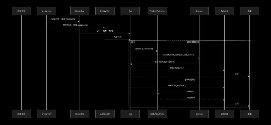
Lhotse 构建了一个严格的分层抽象,每一层解决特定的数据管理问题:物理层负责音频源的统一接入,逻辑层负责训练单元的组织,表示层负责特征的计算与存储。这种分层设计的本质是将数据的物理存储、逻辑组织、计算表示完全解耦,使得每一层可以独立优化和扩展。
Recording 是对完整音频文件的抽象,但其核心价值在于对音频源的封装。在实际生产环境中,音频数据可能存储于本地磁盘、网络文件系统、云存储桶,甚至需要通过流媒体协议实时获取。Recording 通过 AudioSource 这一内部抽象,将音频源的物理位置和访问方式统一为三种类型:文件型、命令型和 URL 型。
文件型直接映射到本地或挂载的文件系统;命令型允许将任意可执行命令的输出作为音频源,这为实时解码和管道处理提供了可能;URL 型则支持从 HTTP 等协议直接拉取音频数据。这种设计的精妙之处在于,上层调用者完全不需要关心音频的物理来源,只需通过统一的接口请求特定时间段的音频数据即可。
Cut 是 Lhotse 最具革命性的抽象,它代表一个可以独立用于训练的最小音频单元。这个单元可能来自原始录音的一个时间片段,也可能是多个音频片段混合后的结果,甚至是经过变速变调处理的变换版本。Cut 的本质是对音频信号在时间轴上的逻辑切片,它通过 start 和 duration 两个参数定义了在原始 Recording 中的位置。
更关键的是,Cut 可以包含多个 Supervision 对象,这些 Supervision 记录了该片段内的所有标注信息,包括文本内容、说话人标识、语种等。当一个 Cut 通过 mix 操作与其他 Cut 叠加时,其内部的 Supervision 会自动合并,保证了标注信息与混合音频的同步。这种设计使得复杂的数据增强操作(如加噪、混响)可以在保持标注一致性的前提下无缝进行。
特征提取是语音识别中计算最密集的环节之一。Lhotse 的设计允许特征以预计算方式存储,也可以在线实时提取。预计算的核心优势在于训练时可以避免重复计算,大幅提升数据加载效率;而在线提取则提供了更大的灵活性,允许动态调整特征参数或在特征域进行数据增强。
特征存储采用 manifest 加数据文件分离的架构。manifest 是 JSONL 格式的元数据文件,记录了每个特征片段的长度、帧移、存储路径等信息;实际的特征数据则通过 lilcom 等压缩算法存储为独立的二进制文件。这种设计既保证了元数据的可读性和可移植性,又实现了特征数据的高效压缩和随机访问。
Lhotse 贯穿始终的设计原则是延迟加载。当构建 RecordingSet 或 CutSet 时,系统仅读取 JSONL 格式的 manifest 文件,不触碰任何实际音频数据。音频的读取发生在明确的 load_audio 调用时,特征的提取发生在 compute_features 调用时,特征的加载发生在 dataset 的 getitem 调用时。
这种惰性计算策略带来了两个关键优势:首先,构建超大规模数据集时内存消耗极低,可以处理数百万条音频的元数据;其次,数据处理流程具有高度的可组合性,可以在不实际加载数据的情况下进行 Cut 的切分、混合、过滤等操作。
Lhotse 为 Cut 设计了一套完整的操作原语,这些原语构成了数据处理的基础算子集。截取操作可以从 Cut 中提取子片段;填充操作用于对齐不同长度的 Cut;混合操作将多个 Cut 的音频叠加并合并标注;映射操作允许对音频波形应用任意函数变换。
这些操作原语的一个重要特性是可组合性。例如,通过组合截取和混合,可以实现语音与噪声的任意信噪比混合;通过组合映射和截取,可以实现语音变速后保持标注对齐。更重要的是,这些操作都是声明式的,它们返回新的 Cut 对象而不实际执行,直到最终需要数据时才触发真正的计算。
特征提取模块采用插件化设计,每种特征类型都实现统一的 FeatureExtractor 接口。该接口定义了 extract 方法用于波形到特征的转换,以及 frame_shift 属性用于时间对齐。这种设计使得添加新的特征类型变得非常简单,只需继承基类并实现核心算法即可。
Lhotse 内置了 FBank、MFCC、Spectrogram 等常用特征提取器,但更重要的是,它允许用户无缝切换计算后端。同一套特征提取代码,可以基于 torchaudio、kaldifeat 或 librosa 实现,系统根据实际安装的库自动选择最优后端。这种设计确保了在科研和生产环境之间的平滑迁移。
Lhotse 的 Dataset 不是简单的特征读取器,而是一个完整的特征工程流水线。当 PyTorch 的 DataLoader 请求一个 batch 的数据时,Dataset 执行以下操作:从 sampler 接收一批 Cut,并行加载对应的特征矩阵,根据 batch 内最长序列进行填充,构建用于 CTC 或 Transducer 损失的 supervision 信息,应用特征域的数据增强(如 SpecAugment),最后将处理好的张量返回给模型。
这种设计的核心价值在于,它将所有特征工程操作都封装在 Dataset 内部,使得训练脚本保持简洁。同时,由于这些操作在 PyTorch 的 DataLoader 工作进程中执行,可以充分利用多核 CPU 进行并行处理,不会阻塞 GPU 训练。
传统的 DataLoader 基于固定 batch size 进行数据组织,但在语音识别中,音频时长差异极大,固定 batch size 会导致 GPU 利用率严重不均。Lhotse 的 DynamicBucketingSampler 采用基于时长的动态批构建策略。
其原理是:将 Cut 按时长分布划分为多个桶(buckets),在每个桶内按照时长排序,然后从各个桶中轮流取出 Cut 组成 batch,确保每个 batch 的总时长不超过预设阈值。这种策略既保证了 batch 内时长的相对均匀,又通过跨桶采样保持了数据的随机性。在 LibriSpeech 等数据集上,动态批构建可以将训练吞吐量提升 3-5 倍。
SpecAugment 是端到端语音识别中最重要的数据增强技术。Lhotse 的实现在设计上考虑了与 CTC/Transducer 损失的兼容性:增强操作需要感知每个样本的有效区域,避免在 padding 部分施加掩蔽。
具体实现时,Dataset 会为每个 batch 构建 supervision_segments 张量,记录每个标注在 batch 中的位置和范围。SpecAugment 模块根据这些信息,只对有效语音区域进行时间和频率掩蔽,而 padding 部分保持不变。这种设计确保了增强操作不会引入虚假的梯度信号。
大规模语音训练面临的核心挑战是 I/O 瓶颈。Lhotse 通过多级缓存和预取机制来缓解这一问题。在特征存储层面,lilcom 压缩算法将特征矩阵压缩至原始大小的 1/3 左右,大幅减少磁盘读取量;在数据加载层面,Dataset 使用多线程并行加载特征文件;在训练循环层面,DataLoader 的 prefetch_factor 参数允许提前加载后续 batch,掩盖 I/O 延迟。
一、音频数据读取:从物理信号到内存张量
1.1 原理篇:声音的数字化
1.1.1 模拟信号 → 数字信号
麦克风采集到的是连续的声音波形(模拟信号),计算机必须将其转换为离散的数字序列。这个过程涉及两个核心参数:
1 2 3 4 5 6 7 8 9 10 11 # 假设一段语音:# 频率:1000Hz(1kHz)# 时长:0.1秒# 采样率 16kHz:每秒采集16000个点# 采样点数 = 16000 * 0.1 = 1600个采样点samples_16k = [0.23, -0.15, 0.08, ...] # 长度1600# 采样率 8kHz:每秒采集8000个点# 采样点数 = 8000 * 0.1 = 800个采样点samples_8k = [0.23, -0.15, 0.08, ...] # 长度800
奈奎斯特采样定理:采样率必须 ≥ 信号最高频率的2倍。语音最高频率约8kHz,所以电话用8kHz,语音识别常用16kHz。
1.1.2 量化精度
每个采样点用多少位二进制表示:
1 2 3 4 # 16-bit 量化:每个点用16位整数表示,范围 -32768 ~ 32767# 浮点表示:通常归一化到 [-1.0, 1.0]pcm_int16 = 32767 * 0.23 # 7536pcm_float32 = 0.23 # 直接浮点
1.1.3 多通道音频
1 2 3 4 5 6 7 8 # 单声道 (Mono): shape (1, N)mono = np.array([[0.23, -0.15, 0.08]])# 双声道 (Stereo): shape (2, N)stereo = np.array([ [0.23, -0.15, 0.08], # 左声道 [0.21, -0.13, 0.07] # 右声道])
1.2 源码篇:Lhotse 的实现
1.2.1 核心数据结构 AudioSource
源码:lhotse/audio/__init__.py
1 2 3 4 5 6 7 8 9 10 11 12 13 14 15 16 17 18 19 20 21 22 23 24 @dataclassclass AudioSource: """音频源的抽象表示""" type: str # 'file', 'command', 'url' path: str # 路径或命令 channels: Union[int, List[int]] # 要读取的通道 def load_audio( self, offset: float = 0.0, # 起始时间(秒) duration: Optional[float] = None # 时长(秒) ) -> np.ndarray: """ 核心方法:将音频源转换为numpy数组 返回形状: (num_channels, num_samples) """ if self.type == 'file': return _load_audio_file(self.path, offset, duration, self.channels) elif self.type == 'command': return _load_audio_command(self.path, offset, duration, self.channels) elif self.type == 'url': return _load_audio_url(self.path, offset, duration, self.channels) else: raise ValueError(f"Unknown audio source type: {self.type}")
1.2.2 实际读取后端
源码:lhotse/audio/backend.py
1 2 3 4 5 6 7 8 9 10 11 12 13 14 15 16 17 18 19 20 21 22 23 24 25 26 27 28 29 30 31 32 33 34 35 36 37 38 39 40 41 42 43 44 45 46 47 48 49 50 51 52 53 54 55 56 57 58 59 60 61 62 63 64 def _load_audio_file( path: str, offset: float = 0.0, duration: Optional[float] = None, channels: Optional[Union[int, List[int]]] = None) -> np.ndarray: """ 多后端音频读取实现 """ # ---- 策略1: 用 torchaudio (最快) ---- try: import torchaudio # 获取音频信息 info = torchaudio.info(path) # 计算帧偏移和帧数 frame_offset = int(offset * info.sample_rate) num_frames = int(duration * info.sample_rate) if duration else -1 # 读取指定片段 waveform, sr = torchaudio.load( path, frame_offset=frame_offset, num_frames=num_frames ) # 选择指定通道 if channels is not None: if isinstance(channels, int): waveform = waveform[channels:channels+1] else: waveform = waveform[channels] return waveform.numpy() except Exception as e1: # ---- 策略2: 用 librosa (支持更多格式) ---- try: import librosa samples, sr = librosa.load( path, sr=None, # 保持原始采样率 offset=offset, duration=duration, mono=False # 保留多通道 ) # librosa返回形状 (T, C),转成 (C, T) if samples.ndim == 1: samples = samples[np.newaxis, :] else: samples = samples.T # 选择指定通道 if channels is not None: if isinstance(channels, int): samples = samples[channels:channels+1] else: samples = samples[channels] return samples except Exception as e2: # ---- 策略3: 用 audioread (最兼容但最慢) ---- return _load_audio_with_audioread(path, offset, duration, channels)
1.2.3 Recording 的封装
源码:lhotse/audio/recording.py
1 2 3 4 5 6 7 8 9 10 11 12 13 14 15 16 17 18 19 20 21 22 23 24 25 26 27 28 29 30 31 32 33 34 35 36 37 38 39 40 41 42 43 44 45 46 47 48 49 @dataclassclass Recording: """一个完整的录音文件""" id: str sources: List[AudioSource] # 可以包含多个源(拼接文件) sampling_rate: int num_samples: int duration: float @classmethod def from_file( cls, path: str, recording_id: Optional[str] = None ) -> 'Recording': """ 从文件创建Recording(只读元数据,不读音频) """ # 用 torchaudio 读取元信息 info = torchaudio.info(path) return cls( id=recording_id or str(uuid.uuid4()), sources=[AudioSource( type='file', path=path, channels=0 # 0表示所有通道 )], sampling_rate=info.sample_rate, num_samples=info.num_frames, duration=info.num_frames / info.sample_rate ) def load_audio( self, channels: Optional[Union[int, List[int]]] = None ) -> np.ndarray: """ 加载整个录音 """ if len(self.sources) == 1: # 单个源 return self.sources[0].load_audio(channels=channels) else: # 多个源需要拼接 audios = [] for source in self.sources: audios.append(source.load_audio(channels=channels)) return np.concatenate(audios, axis=1)
1.3 实战篇:动手操作
1.3.1 从零读取一个音频文件
1 2 3 4 5 6 7 8 9 10 11 12 13 14 15 16 17 18 19 20 21 import numpy as npimport torchaudiofrom lhotse import Recording, AudioSource# 实战1:用 torchaudio 直接读waveform, sr = torchaudio.load('test.wav')print(f"形状: {waveform.shape}") # (通道数, 采样点数)print(f"采样率: {sr}")print(f"时长: {waveform.shape[1] / sr:.2f}秒")print(f"数值范围: [{waveform.min():.3f}, {waveform.max():.3f}]")# 实战2:用 Lhotse Recording 读(只读元信息)rec = Recording.from_file('test.wav')print(f"Recording ID: {rec.id}")print(f"采样率: {rec.sampling_rate}")print(f"总采样点: {rec.num_samples}")print(f"时长: {rec.duration:.2f}秒")# 实战3:实际加载音频(延迟加载)audio = rec.load_audio()print(f"音频形状: {audio.shape}") # (通道数, 采样点数)
1.3.2 处理不同音频源
1 2 3 4 5 6 7 8 9 10 11 12 13 14 15 16 # 实战4:读取音频片段(不加载整个文件)audio_segment = rec.sources[0].load_audio( offset=10.5, # 从10.5秒开始 duration=3.2 # 读3.2秒)print(f"片段形状: {audio_segment.shape}")print(f"实际时长: {audio_segment.shape[1] / rec.sampling_rate:.2f}秒")# 实战5:选择指定通道if audio.shape[0] > 1: # 如果是多通道 # 只读左声道(通道0) left_channel = rec.sources[0].load_audio(channels=0) print(f"左声道形状: {left_channel.shape}") # 只读指定通道组合 selected = rec.sources[0].load_audio(channels=[0, 1]) # 前两个通道
1.3.3 理解采样率和量化
1 2 3 4 5 6 7 8 9 10 11 12 13 14 15 16 17 18 19 20 21 22 23 24 25 26 27 28 29 30 31 32 33 34 35 36 37 38 39 40 41 42 43 44 45 46 47 # 实战6:观察采样率对数据的影响def analyze_sampling_rate(audio_path): # 读原始音频 wave, sr = torchaudio.load(audio_path) print(f"原始采样率: {sr} Hz") print(f"数据点数: {wave.shape[1]}") # 降采样到8kHz(电话音质) wave_8k = torchaudio.functional.resample(wave, sr, 8000) print(f"8kHz 采样: {wave_8k.shape[1]} 点") # 可视化对比(用matplotlib) import matplotlib.pyplot as plt plt.figure(figsize=(12, 4)) # 取前500个点对比 plt.subplot(1, 2, 1) plt.plot(wave[0, :500]) plt.title(f'{sr}Hz 波形') plt.subplot(1, 2, 2) plt.plot(wave_8k[0, :250]) # 8kHz下500点相当于250点 plt.title('8000Hz 波形') plt.show()# 实战7:观察量化精度def analyze_quantization(audio_path): # 读为float32(归一化到[-1, 1]) wave_float, sr = torchaudio.load(audio_path) # 转换为16-bit PCM整数 wave_int16 = (wave_float * 32767).numpy().astype(np.int16) print("Float32范围: [{:.3f}, {:.3f}]".format( wave_float.min(), wave_float.max() )) print("Int16范围: [{}, {}]".format( wave_int16.min(), wave_int16.max() )) # 转回float32看看精度损失 wave_recovered = wave_int16.astype(np.float32) / 32767 mse = np.mean((wave_float.numpy() - wave_recovered) ** 2) print(f"量化误差(MSE): {mse:.6f}")
二、特征提取:从波形到声学特征
2.1 原理篇:语音特征的计算
2.1.1 为什么需要特征?
原始波形有两大问题:
-
1. 维度太高:1秒语音16k个点,100小时就是57.6亿个点 -
2. 信息冗余:相邻采样点高度相关
特征提取的目标:在保持语音识别所需信息的同时,大幅降低维度。
2.1.2 FBank 的计算步骤
第1步:预加重 (Pre-emphasis)
1 2 3 4 5 6 # 原理:提升高频能量,补偿声门脉冲的频谱倾斜# 公式:y[t] = x[t] - α * x[t-1] (α通常取0.97)pre_emphasized = np.append( samples[0], samples[1:] - 0.97 * samples[:-1])
为什么:语音的高频能量通常比低频低,预加重可以平衡频谱,让后续处理更有效。
第2步:分帧 (Framing)
1 2 3 4 5 6 7 8 9 10 11 12 13 14 # 参数:frame_length = 25 # 毫秒frame_shift = 10 # 毫秒sampling_rate = 16000# 转换为采样点数frame_length_samples = int(frame_length * sampling_rate / 1000) # 400点frame_shift_samples = int(frame_shift * sampling_rate / 1000) # 160点# 分帧frames = []for start in range(0, len(samples) - frame_length_samples + 1, frame_shift_samples): frames.append(samples[start:start + frame_length_samples])# frames shape: (num_frames, frame_length)
为什么:语音信号是时变的,但在短时间(10-30ms)内可以认为是平稳的,适合用频谱分析。
第3步:加窗 (Windowing)
1 2 3 4 5 # 汉明窗:减少频谱泄漏window = np.hamming(frame_length_samples)# 公式: w[n] = 0.54 - 0.46 * cos(2πn/(N-1))windowed_frames = frames * window
为什么:直接对截断的信号做FFT会产生频谱泄漏,加窗可以减轻这个问题。
第4步:FFT (快速傅里叶变换)
1 2 3 4 5 6 # 对每一帧做FFTfft_results = np.fft.rfft(windowed_frames, n=512) # 通常补零到2的幂# fft_results shape: (num_frames, 257) 因为rfft只返回正频率# 计算能量谱power_spectrum = np.abs(fft_results) ** 2
物理意义:将信号从时域转换到频域,得到每个频率成分的能量。
第5步:Mel滤波器组
1 2 3 4 5 6 7 8 9 10 11 12 13 14 15 16 17 18 19 20 21 22 23 24 25 def mel_to_hz(mel): """Mel频率转Hz""" return 700 * (10**(mel/2595) - 1)def hz_to_mel(hz): """Hz转Mel频率""" return 2595 * np.log10(1 + hz/700)# 生成Mel刻度上的滤波器组mel_filterbank = []mel_points = np.linspace(hz_to_mel(20), hz_to_mel(8000), 82) # 80个滤波器+2个边界hz_points = mel_to_hz(mel_points)bin_points = np.floor((fft_length + 1) * hz_points / sampling_rate).astype(int)for i in range(80): # 三角形滤波器 filter_ = np.zeros(fft_length//2 + 1) filter_[bin_points[i]:bin_points[i+1]] = np.linspace(0, 1, bin_points[i+1]-bin_points[i]) filter_[bin_points[i+1]:bin_points[i+2]] = np.linspace(1, 0, bin_points[i+2]-bin_points[i+1]) mel_filterbank.append(filter_)mel_filterbank = np.array(mel_filterbank) # (80, 257)# 应用滤波器组mel_energy = np.dot(power_spectrum, mel_filterbank.T) # (num_frames, 80)
为什么用Mel刻度:人耳对频率的感知是非线性的,低频敏感、高频迟钝。Mel刻度模拟了这种感知特性。
第6步:取对数
1 2 log_mel = 10 * np.log10(mel_energy + 1e-10) # 加小常数避免log(0)# log_mel shape: (num_frames, 80) —— 这就是FBank特征
为什么取对数:人耳对音量的感知也是对数级的,同时可以让特征更符合高斯分布假设。
2.2 源码篇:Lhotse 的 FBank 实现
2.2.1 特征提取器基类
源码:lhotse/features/base.py
1 2 3 4 5 6 7 8 9 10 11 12 13 14 15 16 17 18 19 20 21 22 23 24 25 26 27 28 29 30 31 32 33 34 35 36 37 38 39 40 41 42 43 44 45 46 47 48 49 50 51 52 53 54 55 56 57 class FeatureExtractor(ABC): """所有特征提取器的抽象基类""" def __init__(self, config: Optional[Any] = None): self.config = config or self.default_config() @abstractmethod def extract(self, samples: np.ndarray, sampling_rate: int) -> np.ndarray: """ 核心抽象方法:子类必须实现具体的特征计算 输入: samples (C, T) 输出: feats (T', F) """ pass @property @abstractmethod def frame_shift(self) -> float: """帧移(秒)""" pass def extract_from_samples_and_store( self, samples: np.ndarray, storage: 'FeaturesWriter', sampling_rate: int, augment_fn: Optional[Callable] = None ) -> 'Features': """ 完整的提取和存储流水线 """ # 1. 波形域增强(可选) if augment_fn is not None: samples = augment_fn(samples) # 2. 特征提取 feats = self.extract(samples, sampling_rate) # 3. 存储特征 storage_key = storage.write( self._get_storage_key(), feats ) # 4. 返回特征manifest return Features( type=self.name, num_frames=feats.shape[0], num_features=feats.shape[1], frame_shift=self.frame_shift, sampling_rate=sampling_rate, storage_path=storage_key, storage_type=storage.name, start=0, duration=feats.shape[0] * self.frame_shift, recording_id=self.recording_id )
2.2.2 FBank 的具体实现
源码:lhotse/features/fbank.py
1 2 3 4 5 6 7 8 9 10 11 12 13 14 15 16 17 18 19 20 21 22 23 24 25 26 27 28 29 30 31 32 33 34 35 36 37 38 39 40 41 42 43 44 45 46 47 48 49 50 51 52 53 54 55 56 57 58 59 class Fbank(FeatureExtractor): """FBank特征提取器""" name = 'fbank' def __init__(self, config: Optional['FbankConfig'] = None): super().__init__(config) self.config = config or FbankConfig() # 初始化kaldifeat的Fbank import kaldifeat opts = kaldifeat.FbankOptions() opts.frame_opts.samp_freq = self.config.sampling_rate opts.frame_opts.frame_length_ms = self.config.frame_length_ms opts.frame_opts.frame_shift_ms = self.config.frame_shift_ms opts.mel_opts.num_bins = self.config.num_mel_bins opts.mel_opts.low_freq = self.config.low_freq opts.mel_opts.high_freq = self.config.high_freq opts.device = torch.device('cpu') self.extractor = kaldifeat.Fbank(opts) @property def frame_shift(self) -> float: """返回帧移(秒)""" return self.config.frame_shift_ms / 1000.0 def extract(self, samples: np.ndarray, sampling_rate: int) -> np.ndarray: """ 提取FBank特征 参数: samples: (C, T) 的numpy数组 sampling_rate: 采样率 返回: (T', F) 的特征矩阵 """ # 1. 转换为torch tensor samples = torch.from_numpy(samples).float() # 2. 如果需要,重采样 if sampling_rate != self.config.sampling_rate: samples = torchaudio.functional.resample( samples, sampling_rate, self.config.sampling_rate ) # 3. 调用kaldifeat计算特征 # kaldifeat期望输入 (C, T) feats = self.extractor(samples) # (T', F) # 4. 取对数(如果需要) if self.config.use_log: feats = torch.log(torch.clamp(feats, min=1e-10)) # 5. 返回numpy数组 return feats.numpy()
2.2.3 特征存储
源码:lhotse/features/io.py
1 2 3 4 5 6 7 8 9 10 11 12 13 14 15 16 17 18 19 20 21 22 23 24 25 26 27 28 29 30 31 32 class LilcomFilesWriter(FeaturesWriter): """ 用lilcom压缩存储特征 lilcom是专门为语音特征设计的压缩算法,压缩率约3倍 """ name = 'lilcom' def __init__(self, storage_path: Path): self.storage_path = Path(storage_path) self.storage_path.mkdir(parents=True, exist_ok=True) def write(self, key: str, feats: np.ndarray) -> str: """ 写入特征文件 返回存储路径 """ import lilcom # 压缩特征 compressed = lilcom.compress( feats.T, # lilcom期望 (F, T) tick_power=self.config.tick_power, dither=self.config.dither ) # 写入文件 file_path = self.storage_path / f"{key}.llc" with open(file_path, 'wb') as f: f.write(compressed) return str(file_path)
2.3 实战篇:动手提取特征
2.3.1 手动实现FBank(理解原理)
1 2 3 4 5 6 7 8 9 10 11 12 13 14 15 16 17 18 19 20 21 22 23 24 25 26 27 28 29 30 31 32 33 34 35 36 37 38 39 40 41 42 43 44 45 46 47 48 49 50 51 52 53 54 55 56 57 58 59 60 61 62 63 64 65 66 67 68 69 70 71 72 73 74 75 import numpy as npimport librosaimport matplotlib.pyplot as pltdef manual_fbank(audio_path): """ 手动实现FBank计算,一步步看数据变化 """ # 1. 读音频 samples, sr = librosa.load(audio_path, sr=16000, mono=True) print(f"1. 原始波形: shape {samples.shape}, 范围 [{samples.min():.3f}, {samples.max():.3f}]") # 2. 预加重 pre_emphasis = 0.97 samples_pre = np.append(samples[0], samples[1:] - pre_emphasis * samples[:-1]) print(f"2. 预加重后: 范围 [{samples_pre.min():.3f}, {samples_pre.max():.3f}]") # 3. 分帧参数 frame_length = int(0.025 * sr) # 25ms frame_shift = int(0.010 * sr) # 10ms n_fft = 512 frames = librosa.util.frame( samples_pre, frame_length=frame_length, hop_length=frame_shift ).T # (num_frames, frame_length) print(f"3. 分帧后: {frames.shape[0]}帧, 每帧{frame_length}点") # 4. 加窗 window = np.hamming(frame_length) frames_windowed = frames * window # 5. FFT fft = np.fft.rfft(frames_windowed, n=n_fft) power = np.abs(fft) ** 2 print(f"4. FFT后: {power.shape[0]}帧, {power.shape[1]}频点") # 6. Mel滤波 mel_basis = librosa.filters.mel(sr=sr, n_fft=n_fft, n_mels=80) mel_energy = np.dot(power, mel_basis.T) print(f"5. Mel滤波后: {mel_energy.shape} (帧数, Mel维度)") # 7. 取对数 log_mel = 10 * np.log10(mel_energy + 1e-10) print(f"6. FBank特征: {log_mel.shape}") return log_mel, frames, power, mel_energy# 执行fbank, frames, power, mel_energy = manual_fbank('test.wav')# 可视化每一步plt.figure(figsize=(15, 10))plt.subplot(4, 1, 1)plt.plot(frames[0]) # 第一帧波形plt.title('第1帧波形(加窗前)')plt.subplot(4, 1, 2)plt.plot(np.log10(power[0] + 1e-10)) # 第一帧频谱plt.title('第1帧频谱(对数坐标)')plt.subplot(4, 1, 3)plt.imshow(mel_energy.T, aspect='auto', origin='lower')plt.title('Mel能量谱')plt.colorbar()plt.subplot(4, 1, 4)plt.imshow(fbank.T, aspect='auto', origin='lower')plt.title('FBank特征')plt.colorbar()plt.tight_layout()plt.show()
2.3.2 用Lhotse提取特征
1 2 3 4 5 6 7 8 9 10 11 12 13 14 15 16 17 18 19 20 21 22 23 24 25 26 27 28 29 30 31 32 33 34 35 36 37 from lhotse import Recordingfrom lhotse.features import Fbank, FbankConfigfrom lhotse.features.io import LilcomFilesWriterimport tempfile# 1. 创建Recordingrec = Recording.from_file('test.wav')# 2. 配置FBank提取器config = FbankConfig( sampling_rate=16000, frame_length_ms=25, frame_shift_ms=10, num_mel_bins=80, low_freq=20, high_freq=7800, use_log=True)extractor = Fbank(config)# 3. 加载音频audio = rec.load_audio()# 4. 提取特征features = extractor.extract(audio, rec.sampling_rate)print(f"特征形状: {features.shape}") # (num_frames, 80)print(f"第一帧: {features[0, :5]}...")# 5. 存储特征with tempfile.TemporaryDirectory() as tmpdir: writer = LilcomFilesWriter(tmpdir) feat_manifest = extractor.extract_from_samples_and_store( samples=audio, storage=writer, sampling_rate=rec.sampling_rate ) print(f"特征已存储: {feat_manifest.storage_path}")
2.3.3 参数对特征的影响
1 2 3 4 5 6 7 8 9 10 11 12 13 14 15 16 17 18 19 20 21 22 23 24 25 26 27 28 29 30 31 def compare_fbank_params(audio_path): """ 比较不同参数下的FBank特征 """ rec = Recording.from_file(audio_path) audio = rec.load_audio() # 不同配置 configs = { 'default': FbankConfig(), '80维': FbankConfig(num_mel_bins=80), '40维': FbankConfig(num_mel_bins=40), '长窗(50ms)': FbankConfig(frame_length_ms=50), '短窗(10ms)': FbankConfig(frame_length_ms=10), '高频截止4k': FbankConfig(high_freq=4000), } fig, axes = plt.subplots(len(configs), 1, figsize=(12, 3*len(configs))) for i, (name, config) in enumerate(configs.items()): extractor = Fbank(config) feats = extractor.extract(audio, rec.sampling_rate) im = axes[i].imshow(feats.T, aspect='auto', origin='lower') axes[i].set_title(f'{name}: {feats.shape}') plt.colorbar(im, ax=axes[i]) plt.tight_layout() plt.show()compare_fbank_params('test.wav')
三、特征工程:从原始特征到训练就绪
3.1 原理篇:为什么要做特征工程
3.1.1 特征分布问题
原始FBank存在两个问题:
1 2 3 4 5 6 7 8 # 1. 不同样本的动态范围不同sample1_fbank = extractor.extract(audio1) # 范围 [-10, 30]sample2_fbank = extractor.extract(audio2) # 范围 [-5, 25]# 2. 特征值分布可能偏态import matplotlib.pyplot as pltplt.hist(sample1_fbank.flatten(), bins=50)plt.title('FBank值分布(通常不服从高斯分布)')
3.1.2 时间维度问题
1 2 3 # 特征只包含当前帧信息,没有动态信息frame_t = fbank[t] # 只代表当前时刻frame_t_minus_1 = fbank[t-1] # 前后帧的关系没利用
3.1.3 过拟合问题
训练时如果每次都看到相同的特征,模型容易记住而不是学习。
3.2 源码篇:Lhotse 的特征工程实现
3.2.1 CMVN(倒谱均值方差归一化)
源码:lhotse/dataset/signal_transforms.py
1 2 3 4 5 6 7 8 9 10 11 12 13 14 15 16 17 18 19 20 21 22 23 24 25 26 27 28 29 30 31 32 33 34 35 36 37 38 39 40 41 42 43 44 45 46 47 48 49 50 51 52 53 54 55 56 class GlobalMVN(torch.nn.Module): """ 全局倒谱均值方差归一化 让特征服从均值为0,方差为1的分布 """ def __init__( self, norm_means: bool = True, # 是否减均值 norm_vars: bool = False, # 是否除方差 eps: float = 1e-10 ): super().__init__() self.norm_means = norm_means self.norm_vars = norm_vars self.eps = eps def forward(self, features: torch.Tensor) -> torch.Tensor: """ 参数: features: (batch_size, num_frames, num_features) 返回: 归一化后的特征 """ if not (self.norm_means or self.norm_vars): return features # 计算全局统计量 if self.norm_means: # 对所有样本和所有帧求均值 mean = features.mean(dim=(0, 1), keepdim=True) features = features - mean if self.norm_vars: # 计算标准差 std = features.std(dim=(0, 1), keepdim=True) features = features / (std + self.eps) return featuresclass UtteranceMVN(torch.nn.Module): """ 句内归一化(每句话自己归一化) 用于在线场景,不依赖全局统计量 """ def forward(self, features: torch.Tensor) -> torch.Tensor: """ 对每句话自己做归一化 """ # 对每个样本独立计算均值和方差 mean = features.mean(dim=1, keepdim=True) std = features.std(dim=1, keepdim=True) return (features - mean) / (std + self.eps)
3.2.2 Delta 动态特征
源码:lhotse/features/base.py
1 2 3 4 5 6 7 8 9 10 11 12 13 14 15 16 17 18 19 20 21 22 23 24 25 26 27 28 29 30 31 32 33 34 35 36 37 38 39 40 41 42 43 44 45 46 47 48 49 50 51 52 53 54 55 56 57 58 59 60 61 62 63 64 65 66 67 68 69 70 71 72 73 74 75 76 77 78 79 80 81 82 83 84 85 86 87 88 89 90 91 92 93 94 def compute_deltas( feats: np.ndarray, order: int = 2, window: int = 2) -> np.ndarray: """ 计算动态特征 参数: feats: (T, F) 特征矩阵 order: 差分阶数(1或2) window: 窗口大小 返回: (T, F * (order + 1)) 拼接后的特征 """ from scipy.signal import lfilter # 初始化 T, F = feats.shape deltas = [feats] # 滤波器系数(简单差分) window_weights = np.arange(-window, window + 1) window_weights = window_weights / (window_weights ** 2).sum() # 一阶差分 delta1 = np.zeros_like(feats) # 用滤波器计算差分 for f in range(F): delta1[:, f] = lfilter(window_weights, 1, feats[:, f]) deltas.append(delta1) if order >= 2: # 二阶差分(对一阶差分再做一次) delta2 = np.zeros_like(feats) for f in range(F): delta2[:, f] = lfilter(window_weights, 1, delta1[:, f]) deltas.append(delta2) # 沿特征维拼接 return np.concatenate(deltas, axis=1)class DeltaDeltas(torch.nn.Module): """PyTorch版本的Delta计算""" def __init__(self, order: int = 2, window: int = 2): super().__init__() self.order = order self.window = window # 预计算滤波器系数 self.register_buffer( 'weights', self._create_weights(window, order) ) def _create_weights(self, window: int, order: int): """创建差分滤波器系数""" weights = [] for o in range(order + 1): if o == 0: w = torch.zeros(2*window + 1) w[window] = 1.0 else: w = torch.arange(-window, window + 1).float() w = w / (w ** 2).sum() weights.append(w) return torch.stack(weights) def forward(self, features: torch.Tensor) -> torch.Tensor: """ 输入: (B, T, F) 输出: (B, T, F * (order+1)) """ B, T, F = features.shape results = [] for o in range(self.order + 1): # 对每个特征维度应用卷积 weight = self.weights[o] # (2*window+1) # 用conv1d实现差分 feat_o = torch.nn.functional.conv1d( features.transpose(1, 2), # (B, F, T) weight.view(1, 1, -1).repeat(F, 1, 1), # (F, 1, kernel) padding=self.window, groups=F ) # (B, F, T) -> (B, T, F) results.append(feat_o.transpose(1, 2)) # 沿最后一维拼接 return torch.cat(results, dim=-1)
3.2.3 SpecAugment 实现
源码:lhotse/dataset/signal_transforms.py
1 2 3 4 5 6 7 8 9 10 11 12 13 14 15 16 17 18 19 20 21 22 23 24 25 26 27 28 29 30 31 32 33 34 35 36 37 38 39 40 41 42 43 44 45 46 47 48 49 50 51 52 53 54 55 56 57 58 59 60 61 62 63 64 65 66 67 68 69 70 71 72 73 74 75 76 77 78 79 80 81 82 83 84 85 86 87 88 89 90 91 92 93 94 95 96 97 98 99 class SpecAugment(torch.nn.Module): """ SpecAugment: 一种简单的数据增强方法 论文: https://arxiv.org/abs/1904.08779 """ def __init__( self, num_frame_masks: int = 2, # 时间掩蔽次数 frames_mask_size: int = 10, # 时间掩蔽长度(帧数) num_feature_masks: int = 2, # 频率掩蔽次数 feature_mask_size: int = 5, # 频率掩蔽长度(维度数) p: float = 1.0 # 应用概率 ): super().__init__() self.num_frame_masks = num_frame_masks self.frames_mask_size = frames_mask_size self.num_feature_masks = num_feature_masks self.feature_mask_size = feature_mask_size self.p = p def forward( self, features: torch.Tensor, supervision_segments: Optional[torch.Tensor] = None ) -> torch.Tensor: """ 参数: features: (B, T, F) supervision_segments: (N, 3) [batch_idx, start_frame, num_frames] 返回: 增强后的特征 """ if not self.training or torch.rand(1) > self.p: return features if supervision_segments is not None: # 只在有效语音区域做增强 return self._apply_masks_with_supervision(features, supervision_segments) else: # 对整个特征做增强 return self._apply_masks(features) def _apply_masks(self, features: torch.Tensor) -> torch.Tensor: """对整个特征应用掩蔽""" B, T, F = features.shape for _ in range(self.num_frame_masks): # 时间掩蔽 mask_len = min(self.frames_mask_size, T - 1) mask_start = torch.randint(0, T - mask_len, (1,)).item() features[:, mask_start:mask_start+mask_len, :] = 0 for _ in range(self.num_feature_masks): # 频率掩蔽 mask_len = min(self.feature_mask_size, F - 1) mask_start = torch.randint(0, F - mask_len, (1,)).item() features[:, :, mask_start:mask_start+mask_len] = 0 return features def _apply_masks_with_supervision( self, features: torch.Tensor, segments: torch.Tensor ) -> torch.Tensor: """ 只在有语音的区域做增强 segments: (N, 3) [batch_idx, start, duration] """ B, T, F = features.shape result = features.clone() for seg in segments: b, s, d = seg.tolist() s = int(s) d = int(d) # 在这个segment上做增强 segment = result[b, s:s+d, :] # 时间掩蔽 for _ in range(self.num_frame_masks): if d <= self.frames_mask_size: continue mask_len = min(self.frames_mask_size, d - 1) mask_start = torch.randint(0, d - mask_len, (1,)).item() segment[mask_start:mask_start+mask_len, :] = 0 # 频率掩蔽 for _ in range(self.num_feature_masks): mask_len = min(self.feature_mask_size, F - 1) mask_start = torch.randint(0, F - mask_len, (1,)).item() segment[:, mask_start:mask_start+mask_len] = 0 result[b, s:s+d, :] = segment return result
3.3 实战篇:特征工程实践
3.3.1 完整特征处理流水线
1 2 3 4 5 6 7 8 9 10 11 12 13 14 15 16 17 18 19 20 21 22 23 24 25 26 27 28 29 30 31 32 33 34 35 36 37 38 39 40 41 42 43 44 45 46 47 48 49 50 51 52 53 54 55 56 57 58 59 60 61 62 63 64 65 66 67 68 69 70 71 72 73 74 75 76 77 78 79 80 81 82 83 84 85 86 87 88 89 90 91 92 93 94 95 96 97 98 99 100 101 102 103 104 import torchfrom lhotse import CutSet, Fbankfrom lhotse.dataset import K2SpeechRecognitionDatasetfrom lhotse.dataset.sampling import DynamicBucketingSamplerfrom lhotse.dataset.signal_transforms import GlobalMVN, SpecAugmentclass ASRDataModule: """完整的语音识别数据模块""" def __init__(self, config): self.config = config # 1. 特征提取器 self.feature_extractor = Fbank(config.feature_config) # 2. 特征归一化 self.global_mvn = GlobalMVN( norm_means=True, norm_vars=config.norm_vars ) # 3. 数据增强(只在训练时使用) self.spec_augment = SpecAugment( num_frame_masks=config.num_frame_masks, frames_mask_size=config.frames_mask_size, num_feature_masks=config.num_feature_masks, feature_mask_size=config.feature_mask_size ) def train_dataloader(self): """训练数据加载器""" # 加载cutset cuts = CutSet.from_file(self.config.train_cuts) # 动态批采样器(按时长) sampler = DynamicBucketingSampler( cuts, max_duration=self.config.max_duration, shuffle=True ) # 数据集 dataset = K2SpeechRecognitionDataset( cuts, feature_extractor=self.feature_extractor, global_mvn=self.global_mvn, spec_augment=self.spec_augment # 训练时启用 ) return torch.utils.data.DataLoader( dataset, batch_sampler=sampler, num_workers=self.config.num_workers ) def valid_dataloader(self): """验证数据加载器(不使用增强)""" cuts = CutSet.from_file(self.config.valid_cuts) sampler = DynamicBucketingSampler( cuts, max_duration=self.config.max_duration, shuffle=False ) dataset = K2SpeechRecognitionDataset( cuts, feature_extractor=self.feature_extractor, global_mvn=self.global_mvn, spec_augment=None # 验证时不用增强 ) return torch.utils.data.DataLoader( dataset, batch_sampler=sampler, num_workers=self.config.num_workers )# 使用示例config = { 'feature_config': FbankConfig( sampling_rate=16000, num_mel_bins=80 ), 'norm_vars': False, 'num_frame_masks': 2, 'frames_mask_size': 10, 'num_feature_masks': 2, 'feature_mask_size': 5, 'max_duration': 200.0, # 每个batch最多200秒 'num_workers': 4}data_module = ASRDataModule(config)train_loader = data_module.train_dataloader()# 看一个batchfor batch in train_loader: features = batch['features'] # (B, T, 80) print(f"Batch特征形状: {features.shape}") print(f"特征范围: [{features.min():.3f}, {features.max():.3f}]") print(f"特征均值: {features.mean():.3f}") print(f"特征标准差: {features.std():.3f}") break
3.3.2 可视化特征工程的效果
1 2 3 4 5 6 7 8 9 10 11 12 13 14 15 16 17 18 19 20 21 22 23 24 25 26 27 28 29 30 31 32 33 34 35 36 37 38 39 40 41 42 43 44 45 46 47 48 49 50 51 52 53 54 55 56 57 58 59 60 61 62 63 64 65 66 67 68 69 70 71 72 73 74 75 76 77 78 79 80 def visualize_feature_pipeline(audio_path): """ 可视化特征处理每个阶段的效果 """ import matplotlib.pyplot as plt from lhotse import Recording from lhotse.features import Fbank from lhotse.dataset.signal_transforms import GlobalMVN, SpecAugment # 1. 加载音频并提取原始FBank rec = Recording.from_file(audio_path) audio = rec.load_audio() extractor = Fbank() raw_fbank = extractor.extract(audio, rec.sampling_rate) raw_fbank = torch.from_numpy(raw_fbank).unsqueeze(0) # (1, T, F) # 2. CMVN归一化 mvn = GlobalMVN(norm_means=True, norm_vars=False) norm_fbank = mvn(raw_fbank) # 3. SpecAugment specaug = SpecAugment( num_frame_masks=2, frames_mask_size=10, num_feature_masks=2, feature_mask_size=5 ) specaug.train() # 启用训练模式 aug_fbank = specaug(norm_fbank) # 可视化 fig, axes = plt.subplots(3, 3, figsize=(15, 12)) # 原始特征 axes[0, 0].imshow(raw_fbank[0].T, aspect='auto', origin='lower') axes[0, 0].set_title('原始FBank') axes[0, 1].hist(raw_fbank[0].flatten(), bins=50) axes[0, 1].set_title('原始分布') axes[0, 2].plot(raw_fbank[0, :, 20].numpy()) # 第20维的时间序列 axes[0, 2].set_title('第20维随时间变化') # 归一化后 axes[1, 0].imshow(norm_fbank[0].T, aspect='auto', origin='lower') axes[1, 0].set_title('CMVN归一化') axes[1, 1].hist(norm_fbank[0].flatten(), bins=50) axes[1, 1].set_title('归一化后分布') axes[1, 2].plot(norm_fbank[0, :, 20].numpy()) axes[1, 2].set_title('归一化后第20维') # 增强后 axes[2, 0].imshow(aug_fbank[0].T, aspect='auto', origin='lower') axes[2, 0].set_title('SpecAugment增强') axes[2, 1].hist(aug_fbank[0].flatten(), bins=50) axes[2, 1].set_title('增强后分布') axes[2, 2].plot(aug_fbank[0, :, 20].numpy()) axes[2, 2].set_title('增强后第20维') plt.tight_layout() plt.show() # 打印统计信息 print("原始特征: 均值={:.3f}, 标准差={:.3f}".format( raw_fbank.mean(), raw_fbank.std() )) print("归一化后: 均值={:.3f}, 标准差={:.3f}".format( norm_fbank.mean(), norm_fbank.std() )) print("增强后: 均值={:.3f}, 标准差={:.3f}".format( aug_fbank.mean(), aug_fbank.std() ))# 执行visualize_feature_pipeline('test.wav')
3.3.3 从零构建完整的数据流
1 2 3 4 5 6 7 8 9 10 11 12 13 14 15 16 17 18 19 20 21 22 23 24 25 26 27 28 29 30 31 32 33 34 35 36 37 38 39 40 41 42 43 44 45 46 47 48 49 50 51 52 53 54 55 56 57 58 59 60 61 62 63 64 65 66 67 68 69 70 71 72 73 74 75 76 77 78 79 80 81 82 83 84 85 86 87 88 89 90 91 92 93 94 95 96 97 98 99 100 101 102 103 104 105 106 107 108 109 110 111 112 113 114 115 116 117 118 119 120 121 122 123 import torchfrom pathlib import Pathfrom lhotse import RecordingSet, SupervisionSet, CutSetfrom lhotse.recipes import prepare_librispeechfrom lhotse.features import Fbank, FbankConfigfrom lhotse.features.io import LilcomFilesWriterfrom lhotse.dataset import K2SpeechRecognitionDatasetfrom lhotse.dataset.sampling import DynamicBucketingSamplerdef build_data_pipeline(data_dir: Path, exp_dir: Path): """ 构建完整的数据处理流水线 """ # ---- 第1步:准备原始数据 ---- print("1. 准备原始数据...") libri = prepare_librispeech( data_dir / 'LibriSpeech', output_dir=exp_dir / 'manifests' ) # 获取训练集和验证集 train_cuts = libri['train-clean-100'] valid_cuts = libri['dev-clean'] print(f"训练集: {len(train_cuts)} 条") print(f"验证集: {len(valid_cuts)} 条") # ---- 第2步:配置特征提取 ---- print("\n2. 配置特征提取...") extractor = Fbank( FbankConfig( sampling_rate=16000, frame_length_ms=25, frame_shift_ms=10, num_mel_bins=80, use_log=True ) ) # ---- 第3步:提取并存储特征 ---- print("\n3. 提取特征...") storage_path = exp_dir / 'feats' storage_path.mkdir(exist_ok=True) # 为训练集提取特征 train_cuts = train_cuts.compute_and_store_features( extractor=extractor, storage_path=storage_path / 'train', num_jobs=4 ) # 为验证集提取特征 valid_cuts = valid_cuts.compute_and_store_features( extractor=extractor, storage_path=storage_path / 'valid', num_jobs=4 ) # 保存带有特征路径的cuts train_cuts.to_file(exp_dir / 'cuts_train.jsonl.gz') valid_cuts.to_file(exp_dir / 'cuts_valid.jsonl.gz') # ---- 第4步:创建PyTorch数据集 ---- print("\n4. 创建数据集...") # 训练集(带数据增强) train_dataset = K2SpeechRecognitionDataset( cuts=train_cuts, global_mvn=True, # 全局归一化 spec_augment=True # 启用SpecAugment ) # 验证集(无增强) valid_dataset = K2SpeechRecognitionDataset( cuts=valid_cuts, global_mvn=True, spec_augment=False ) # ---- 第5步:创建DataLoader ---- print("\n5. 创建DataLoader...") train_sampler = DynamicBucketingSampler( train_cuts, max_duration=200.0, # 每个batch最多200秒音频 shuffle=True ) valid_sampler = DynamicBucketingSampler( valid_cuts, max_duration=200.0, shuffle=False ) train_loader = torch.utils.data.DataLoader( train_dataset, batch_sampler=train_sampler, num_workers=4 ) valid_loader = torch.utils.data.DataLoader( valid_dataset, batch_sampler=valid_sampler, num_workers=4 ) # ---- 第6步:测试数据流 ---- print("\n6. 测试数据流...") for batch in train_loader: features = batch['features'] print(f"Batch特征形状: {features.shape}") print(f"特征均值: {features.mean():.3f}") print(f"特征标准差: {features.std():.3f}") print(f"特征中0值的比例: {(features == 0).float().mean():.3f}") # SpecAugment的掩蔽 break return train_loader, valid_loader# 执行train_loader, valid_loader = build_data_pipeline( data_dir=Path('/path/to/data'), exp_dir=Path('./exp'))
总结:三个阶段的对应关系
|
|
|
|
|
|---|---|---|---|
| 音频读取 |
|
|
|
| 特征提取 |
|
|
|
| 特征工程 |
|
|
|