想学习Word2vec?用Numpy从Scratch开始带你完整过一遍

除了干货，其他什么也没有
手册	安装	自学	练习	合作

▼

2020最新

NumPy中文手册

▲

1、介绍

深度神经网络的原理！

↑点击上方蓝字进入查看↑

最近，我在工作中接触了几个与NLP有关的项目。其中很多都是与单词嵌入（word embedding）有关。在工作中，这些任务大多是借助大名鼎鼎的Python库：gensim来完成的。然而，我决定仅仅借助Python和NumPy从头开始实现一个Word2vec模型，之所以决定重新发明一遍轮子，是因为我想深入学习一下Word2vec，顺便巩固一下Numpy。

2、词语嵌入

我用Numpy编写了一个深度神经网络

↑点击上方蓝字进入查看↑

词语嵌入并没有什么花哨的东西，而是用数字的方式来表示词汇的方法。更确切地说，是将词汇映射到向量的方法。

最直接的方法可以是使用一热编码，将每个字映射到一热向量上。

虽然一热编码很简单，但也有几个缺点。最显著的一个缺点就是不容易用数学的方式来衡量词语之间的关系。

Word2vec是一种神经网络结构，通过在监督分类问题上训练模型来生成词嵌入。

Word2vec方法在Mikolov等人的论文《Efficient Estimation of Word Representations in Vector Space》中首次提出，并被证明在实现单词嵌入方面相当成功，可以用来衡量单词之间的句法和语义相似性。

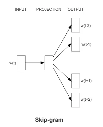
Word2vec (Skip-gram)

在Mikolov et al.,2013中，提出了两种模型架构，即连续字袋模型和Skip-gram模型。我将在本文中深入探讨后者。

为了解释Skip-gram模型，我想起我目前正在阅读的约翰-博格尔的《投资的常识》。

扣除投资成本后，战胜股市注定是一大群人都将失败的游戏。

正如我上面提到的，word2vec模型试图优化的是一个监督分类问题。

更具体地说，给定一个"上下文词"，我们希望训练一个模型，使该模型能够预测一个"目标词"，即在上下文环境具备下出现一个预测的词。

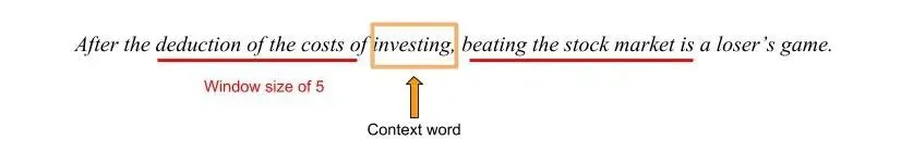
以上面的句子为例，给定语境词"投资"，窗口大小为5，我们希望模型能生成其中一个基础词。(案例中[deduction, of, the costs, beating, stock, market, is]中的一个词)。

模型概述

以下是Mikolov等人2013年的论文中提出的原图。

我做了另一张图，有更多的细节。

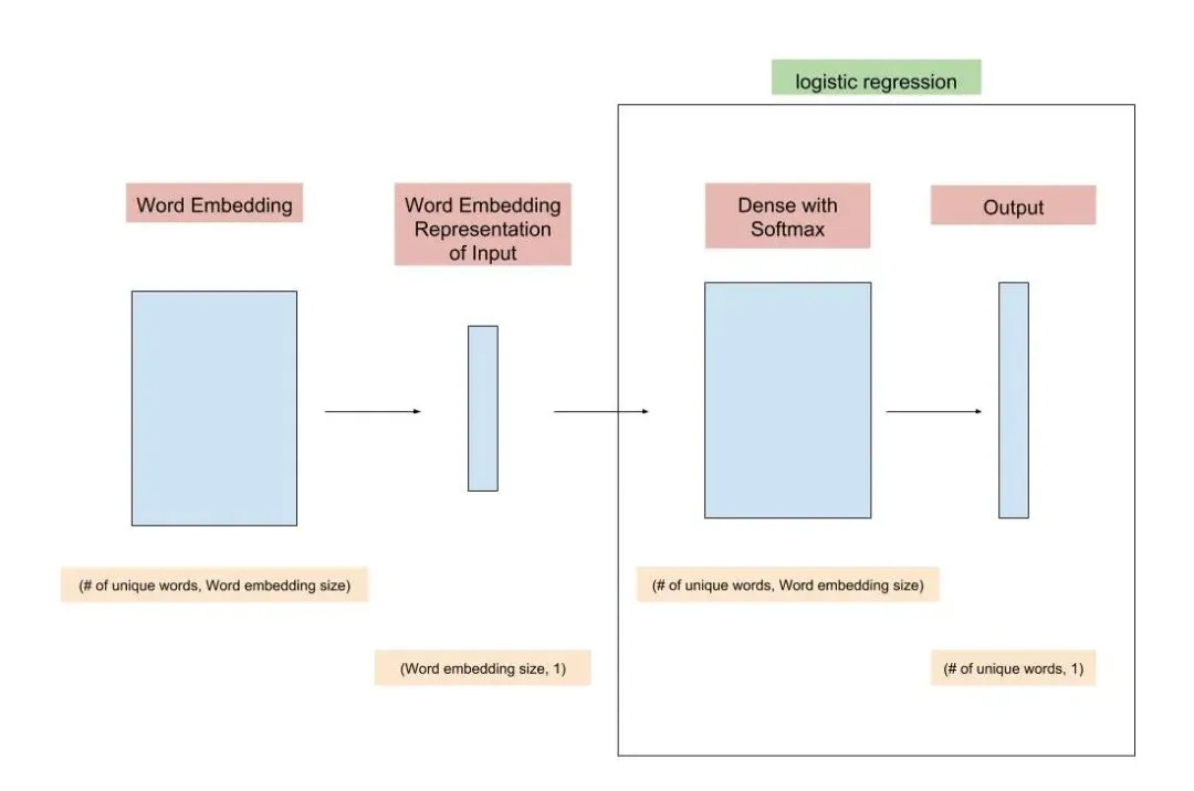
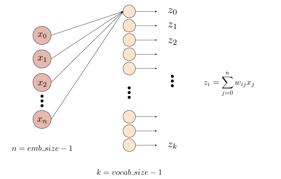
词嵌入层本质上是一个矩阵，其形状为（语料库中唯一词的数量，词嵌入大小）。矩阵的每一行代表语料库中的一个词。词嵌入大小是一个待定的超参数，可以认为是我们希望用多少个特征来代表每个词。模型的后半部分只是一个神经网络形式的逻辑回归。

在训练过程中，单词嵌入层和密集层正在被训练，这样的模型能够在训练过程结束时给定一个上下文单词来预测目标单词。

在用大量的数据来训练这样的模型后，单词嵌入层最终会变成一个单词的表示，可以用数学的方式来展示单词之间的多种酷似关系。有兴趣了解更多细节的朋友可以参考原论文。

3、用python从零开始实现

培训数据的准备

为了生成训练数据，我们首先对文本进行标记。在对文本数据进行标记的时候，有很多技术，比如把出现频率很高或很低的词去掉。我只是用一个简单的检索词来分割文本，因为文章的重点不是标记。

接下来，我们给每个词分配一个整数作为它的id。此外，使用word_to_id和id_to_word来记录映射关系。

最终，我们为模型生成训练数据。对于每个语境词tokens[i]，生成。(tokens[i]，tokens[i-window_size])，...，(tokens[i]，tokens[i-1])，(tokens[i]，tokens[i+1])，...，(tokens[i]，tokens[i+window_size])。以上下文词investing为例，窗口大小为5，我们将生成(investing，deduction)，(investing，of)，(investing，the)，(investing，cost)，(investing，of)，(investing，beating)，(investing，the)，(investing，stock)，(investing，market)，(investing，is)。注：在代码中，训练(x，y)对用单词id表示。

以下是生成训练数据的代码。

import redef tokenize(text):    # obtains tokens with a least 1 alphabet    pattern = re.compile(r'[A-Za-z]+[\w^\']*|[\w^\']*[A-Za-z]+[\w^\']*')    return pattern.findall(text.lower())def mapping(tokens):    word_to_id = dict()    id_to_word = dict()    for i, token in enumerate(set(tokens)):        word_to_id[token] = i        id_to_word[i] = token    return word_to_id, id_to_worddef generate_training_data(tokens, word_to_id, window_size):    N = len(tokens)    X, Y = [], []    for i in range(N):        nbr_inds = list(range(max(0, i - window_size), i)) + \                   list(range(i + 1, min(N, i + window_size + 1)))        for j in nbr_inds:            X.append(word_to_id[tokens[i]])            Y.append(word_to_id[tokens[j]])    X = np.array(X)    X = np.expand_dims(X, axis=0)    Y = np.array(Y)    Y = np.expand_dims(Y, axis=0)    return X, Ydoc = "After the deduction of the costs of investing, " \      "beating the stock market is a loser's game."tokens = tokenize(doc)word_to_id, id_to_word = mapping(tokens)X, Y = generate_training_data(tokens, word_to_id, 3)vocab_size = len(id_to_word)m = Y.shape[1]# turn Y into one hot encodingY_one_hot = np.zeros((vocab_size, m))Y_one_hot[Y.flatten(), np.arange(m)] = 1

训练完整过程

生成训练数据后，我们继续训练模型。和大多数神经网络模型类似，训练word2vec模型的步骤是初始化权重（我们要训练的参数）、向前传播、计算成本、向后传播和更新权重。整个过程会根据我们想要训练的纪元数重复几次迭代。

初始化要训练的参数

模型中有两层需要初始化和训练，即词嵌入层和致密层。

词语嵌入的形状将是（vocab_size，emb_size）。

为什么会这样呢？如果我们想用一个包含 emb_size 元素的向量来表示一个词汇，而我们语料库的词汇总数是 vocab_size，那么我们可以用 vocab_size x emb_size 矩阵来表示所有的词汇，每一行代表一个单词。

密集层的形状将是（vocab_size，emb_size）。

怎么会这样呢？这层中要进行的操作是矩阵乘法。这层的输入将是(emb_size, # 训练实例的数量)，我们希望输出是(vocab_size, # 训练实例的数量)(对于每个单词，我们想知道该单词与给定输入单词一起出现的概率是多少)。注意：我在密集层中不包含偏误。

以下是代码。

def initialize_wrd_emb(vocab_size, emb_size):    """    vocab_size: int. vocabulary size of your corpus or training data    emb_size: int. word embedding size. How many dimensions to represent each vocabulary    """    WRD_EMB = np.random.randn(vocab_size, emb_size) * 0.01    return WRD_EMBdef initialize_dense(input_size, output_size):    """    input_size: int. size of the input to the dense layer    output_szie: int. size of the output out of the dense layer    """    W = np.random.randn(output_size, input_size) * 0.01    return Wdef initialize_parameters(vocab_size, emb_size):    """    initialize all the trianing parameters    """    WRD_EMB = initialize_wrd_emb(vocab_size, emb_size)    W = initialize_dense(emb_size, vocab_size)    parameters = {}    parameters['WRD_EMB'] = WRD_EMB    parameters['W'] = W    return parameters

Forward pass

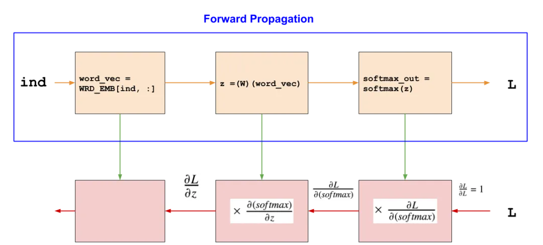
Forward pass有三个步骤，从词嵌入中获得输入词的向量表示，将向量传递给致密层，然后对致密层的输出应用softmax函数。

在一些文献中，输入是以一个一热向量的形式呈现的（比方说一个一热向量，第i个元素为1）。通过将词嵌入矩阵和一热向量相乘，我们可以得到代表输入词的向量。

然而，执行矩阵乘法的结果与选择字嵌入矩阵的第i行基本相同。我们只需选择与输入词相关联的行，就可以节省大量的计算时间。

剩下的过程只是一个多类线性回归模型。

可以用下图来回忆密集层的主要操作。

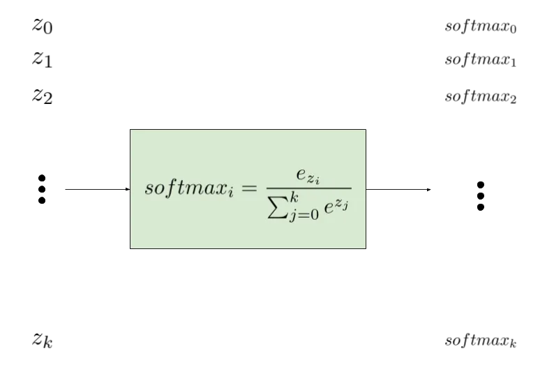
之后，我们将softmax函数应用到密集层的输出中，它给出了每个词出现在给定输入词附近的概率。下面的公式可以用来提醒什么是softmax函数。

以下是Forward pass的代码。

def ind_to_word_vecs(inds, parameters):    """    inds: numpy array. shape: (1, m)    parameters: dict. weights to be trained    """    m = inds.shape[1]    WRD_EMB = parameters['WRD_EMB']    word_vec = WRD_EMB[inds.flatten(), :].T    assert(word_vec.shape == (WRD_EMB.shape[1], m))    return word_vecdef linear_dense(word_vec, parameters):    """    word_vec: numpy array. shape: (emb_size, m)    parameters: dict. weights to be trained    """    m = word_vec.shape[1]    W = parameters['W']    Z = np.dot(W, word_vec)    assert(Z.shape == (W.shape[0], m))    return W, Zdef softmax(Z):    """    Z: output out of the dense layer. shape: (vocab_size, m)    """    softmax_out = np.divide(np.exp(Z), np.sum(np.exp(Z), axis=0, keepdims=True) + 0.001)    assert(softmax_out.shape == Z.shape)    return softmax_outdef forward_propagation(inds, parameters):    word_vec = ind_to_word_vecs(inds, parameters)    W, Z = linear_dense(word_vec, parameters)    softmax_out = softmax(Z)    caches = {}    caches['inds'] = inds    caches['word_vec'] = word_vec    caches['W'] = W    caches['Z'] = Z    return softmax_out, caches

成本的计算(L)

在这里，我们会用交叉熵来计算成本。

以下是成本计算的代码。

def cross_entropy(softmax_out, Y):    """    softmax_out: output out of softmax. shape: (vocab_size, m)    """    m = softmax_out.shape[1]    cost = -(1 / m) * np.sum(np.sum(Y * np.log(softmax_out + 0.001), axis=0, keepdims=True), axis=1)    return cost

Backward pass (Back propagation)

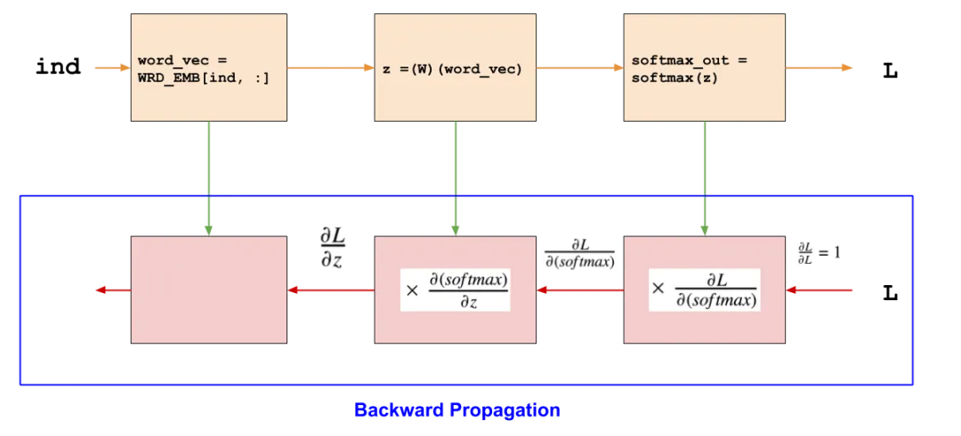在反向传播过程中，我们希望计算可训练权重相对于损失函数的梯度，并更新权重与其相关的梯度。回传播就是用来计算这些梯度的方法。它没有什么花哨的东西，只是微积分中的链式规则。

我们要训练的是密集层和词嵌入层的权重。因此我们需要计算这些权重的梯度。

下一步是用下面的公式更新权重。

以下是Back propagation的代码。

def softmax_backward(Y, softmax_out):    """    Y: labels of training data. shape: (vocab_size, m)    softmax_out: output out of softmax. shape: (vocab_size, m)    """    dL_dZ = softmax_out - Y    assert(dL_dZ.shape == softmax_out.shape)    return dL_dZdef dense_backward(dL_dZ, caches):    """    dL_dZ: shape: (vocab_size, m)    caches: dict. results from each steps of forward propagation    """    W = caches['W']    word_vec = caches['word_vec']    m = word_vec.shape[1]    dL_dW = (1 / m) * np.dot(dL_dZ, word_vec.T)    dL_dword_vec = np.dot(W.T, dL_dZ)    assert(W.shape == dL_dW.shape)    assert(word_vec.shape == dL_dword_vec.shape)    return dL_dW, dL_dword_vecdef backward_propagation(Y, softmax_out, caches):    dL_dZ = softmax_backward(Y, softmax_out)    dL_dW, dL_dword_vec = dense_backward(dL_dZ, caches)    gradients = dict()    gradients['dL_dZ'] = dL_dZ    gradients['dL_dW'] = dL_dW    gradients['dL_dword_vec'] = dL_dword_vec    return gradientsdef update_parameters(parameters, caches, gradients, learning_rate):    vocab_size, emb_size = parameters['WRD_EMB'].shape    inds = caches['inds']    WRD_EMB = parameters['WRD_EMB']    dL_dword_vec = gradients['dL_dword_vec']    m = inds.shape[-1]    WRD_EMB[inds.flatten(), :] -= dL_dword_vec.T * learning_rate    parameters['W'] -= learning_rate * gradients['dL_dW']

注意：你可能会有疑问，为什么dL_dW中有一个1/m的因子，而dL_dword_vec中没有在每个通道中，我们一起处理m个训练例子。

对于密集层中的权重，我们希望用m个梯度下降的平均值来更新它们。对于词向量中的权重，每个向量都有自己的权重，导致自己的梯度下降，所以我们在更新时不需要将m个梯度下降汇总。

模型训练

训练模型时，要重复前向传播、后向传播和权重更新的过程。在训练过程中，每一个纪元后的成本应该有下降的趋势。

以下是训练模型的代码。

def skipgram_model_training(X, Y, vocab_size, emb_size, learning_rate, epochs, batch_size=256, parameters=None, print_cost=True, plot_cost=True):    """    X: Input word indices. shape: (1, m)    Y: One-hot encodeing of output word indices. shape: (vocab_size, m)    vocab_size: vocabulary size of your corpus or training data    emb_size: word embedding size. How many dimensions to represent each vocabulary    learning_rate: alaph in the weight update formula    epochs: how many epochs to train the model    batch_size: size of mini batch    parameters: pre-trained or pre-initialized parameters    print_cost: whether or not to print costs during the training process    """    costs = []    m = X.shape[1]    if parameters is None:        parameters = initialize_parameters(vocab_size, emb_size)    for epoch in range(epochs):        epoch_cost = 0        batch_inds = list(range(0, m, batch_size))        np.random.shuffle(batch_inds)        for i in batch_inds:            X_batch = X[:, i:i+batch_size]            Y_batch = Y[:, i:i+batch_size]            softmax_out, caches = forward_propagation(X_batch, parameters)            gradients = backward_propagation(Y_batch, softmax_out, caches)            update_parameters(parameters, caches, gradients, learning_rate)            cost = cross_entropy(softmax_out, Y_batch)            epoch_cost += np.squeeze(cost)        costs.append(epoch_cost)        if print_cost and epoch % (epochs // 500) == 0:            print("Cost after epoch {}: {}".format(epoch, epoch_cost))        if epoch % (epochs // 100) == 0:            learning_rate *= 0.98    if plot_cost:        plt.plot(np.arange(epochs), costs)        plt.xlabel('# of epochs')        plt.ylabel('cost')    return parameters

总结

用上面例子句子生成的数据训练模型后，窗口大小为3，时间为5000个epochs（简单的学习率衰减），我们可以看到模型可以在给定每个词作为输入词的情况下，输出大多数相邻词。