 夜雨聆风
夜雨聆风系列第 08 篇|阅读时长约 10 分钟关键词:QTL-seq R 包、MutMap、DeepBSA、工具对比
一个现实问题
上一篇文章我们用 Python 从零实现了 BSA 算法——原理懂透了。
但真正做项目时,没人愿意每次都自己写代码。
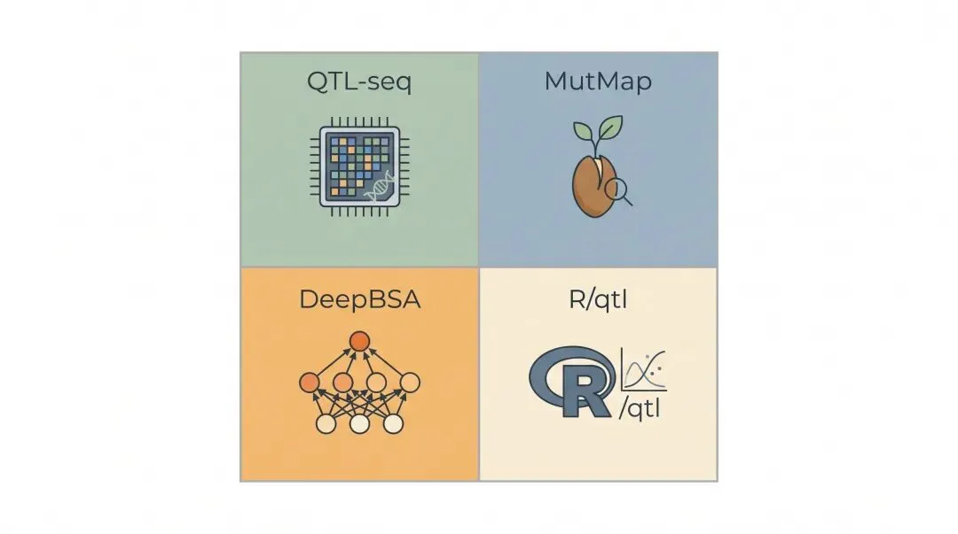
这篇我把 BSA 圈最常用的 3 个工具——QTL-seq、MutMap、DeepBSA——逐个上手演示一遍,最后给一个我自己用的工具组合策略。
一、QTL-seq(R 包版本):最经典的 BSA 工具
1.1 工具背景
出处:Takagi 等 2013 年提出算法 包装:QTL-seq R 包(作者日本人 Sugihara) 现状:BSA 圈引用率最高的工具
1.2 安装
ounter(lineounter(lineounter(lineounter(lineounter(line# R 4.xif (!requireNamespace("devtools", quietly = TRUE))install.packages("devtools")devtools::install_github("bmansfeld/QTLseqr")
1.3 数据准备
QTL-seqr 接受 VCF 文件,但需要特定的列。可以从 VCF 读:
ounter(lineounter(lineounter(lineounter(lineounter(lineounter(lineounter(lineounter(linelibrary(QTLseqr)# 从 VCF 读df <- importFromVCF(vcfFile = "03_variants/final.vcf.gz",chromList = paste0("Chr", 1:12), # 水稻12条染色体filename = NULL)
或者从 CSV 读(自己用 bcftools 提取):
ounter(lineounter(lineounter(line# 提取 BSA 需要的字段bcftools query -f '%CHROM\t%POS\t%REF\t%ALT[\t%AD]\n' \03_variants/final.vcf.gz > snp_data.tsv
1.4 跑 SNP-index
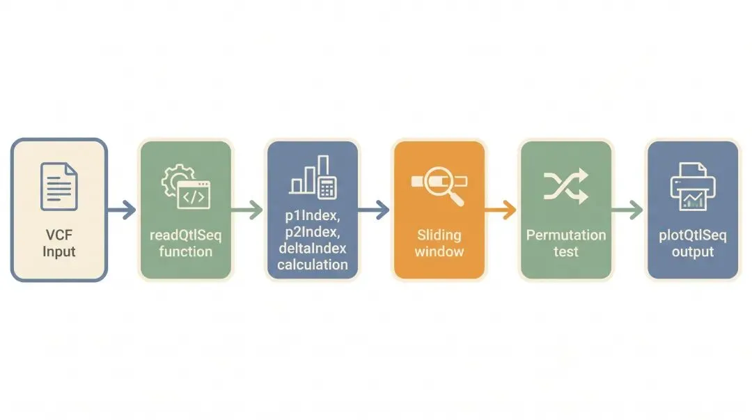
ounter(lineounter(lineounter(lineounter(lineounter(lineounter(lineounter(lineounter(lineounter(lineounter(lineounter(lineounter(lineounter(lineounter(linedf <- runQTLseqAnalysis(SNPset = df,chromList = paste0("Chr", 1:12),popSize = 50, # 每个池的个体数bulkL = "Bulk-L", # 低池样本名前缀bulkH = "Bulk-H", # 高池样本名前缀qtlevel = 0.05, # 显著性水平filter = "all", # 过滤策略interMethod = "dh", # 插值方法windowSize = 1e6, # 窗口大小stepSize = 1e5, # 步长minRawDepth = 10,maxRawDepth = 100)
1.5 画图
ounter(lineounter(lineounter(lineounter(lineounter(lineounter(lineplotQTLStats(SNPset = df,varCol = "deltaSNP",chromList = paste0("Chr", 1:12),threshold = 0.33)
一行出图。但默认样式有点丑,建议加 ggplot2 美化:
ounter(lineounter(lineounter(lineounter(lineounter(lineounter(lineounter(lineounter(lineounter(linelibrary(ggplot2)ggplot(df, aes(x = pos, y = abs(deltaSNP), color = chr)) +geom_point(size = 0.8) +facet_grid(. ~ chr, scales = "free_x", space = "free_x") +geom_hline(yintercept = 0.33, linetype = "dashed", color = "red") +theme_bw() +theme(axis.text.x = element_blank()) +labs(title = "BSA Manhattan Plot (QTL-seqr)",x = "Chromosome", y = "|ΔSNP-index|")
二、MutMap / MutMap+:突变体的福音
2.1 工具背景
出处:Abe 等 2012 年提出 适用:EMS 诱变 / CRISPR 突变体定位 核心思想:跟 BSA 一样,但直接拿突变池跟亲本比,不建群体
2.2 MutMap vs MutMap+ 区别
| MutMap+ |
MutMap+ 比 MutMap 更灵敏——因为用了 F2 中野生型个体做参考,能过滤掉非目标 SNP。
2.3 MutMap 计算逻辑
本质就是:
ounter(lineSNP-index = alt_in_mutant / (ref_in_mutant + alt_in_mutant)
期望:目标位点 SNP-index ≈ 1(突变纯合),非目标位点 ≈ 0.5。
2.4 用 R 实现 MutMap 流程
ounter(lineounter(lineounter(lineounter(lineounter(lineounter(lineounter(lineounter(lineounter(lineounter(lineounter(lineounter(lineounter(lineounter(lineounter(lineounter(lineounter(lineounter(lineounter(lineounter(line# MutMap 用 SNP-index,画滑窗图mutmap_df <- data.frame(chr = df$CHROM,pos = df$POS,snp_index = df$alt / (df$ref + df$alt))# 滑窗library(zoo)mutmap_df$win_mean <- zoo::rollmean(mutmap_df$snp_index,k = 100, # 100 个 SNP 一个窗口fill = NA)# 画图plot(mutmap_df$pos, mutmap_df$win_mean,pch = 19, cex = 0.3, col = "steelblue",xlab = "Position", ylab = "SNP-index (MutMap)")abline(h = 0.9, col = "red", lty = 2)
2.5 MutMap 的特殊过滤:EMS 背景过滤
EMS 诱变的 SNP 分布有个特点——C→T 和 G→A 转换占绝大多数。
ounter(lineounter(lineounter(lineounter(line# 用 bcftools 过滤出 EMS 相关的转换bcftools view -i 'TYPE="snp"' final.vcf.gz | \bcftools filter -i '(REF="C" && ALT="T") || (REF="G" && ALT="A")' \-Oz -o ems_snps.vcf.gz
这样能去掉非 EMS 背景噪音。
三、DeepBSA:深度学习新派工具
3.1 工具背景
出处:2022 年华中农业大学李林课题组(Molecular Plant) 核心:用 CNN 神经网络做 BSA 信号识别 优势:号称能在小群体(< 20 株/池)下保持定位能力
3.2 安装
ounter(lineounter(lineounter(linegit clone https://github.com/yongdeng34/DeepBSA.gitcd DeepBSApip install -r requirements.txt
3.3 跑 DeepBSA
ounter(lineounter(lineounter(lineounter(lineounter(lineounter(linepython DeepBSA.py \--vcf 03_variants/final.vcf.gz \--high-bulk bulk_H_1,bulk_H_2 \--low-bulk bulk_L_1,bulk_L_2 \--window 1000000 \--output deepbsa_results/
跑完会输出一个 result.txt,包含每个窗口的预测分数和对应的候选区间。
3.4 怎么看 DeepBSA 结果
ounter(lineounter(lineounter(lineounter(lineounter(lineounter(lineounter(lineounter(lineounter(lineounter(lineounter(lineounter(lineounter(lineounter(lineounter(lineimport pandas as pdimport matplotlib.pyplot as pltresult = pd.read_csv("deepbsa_results/result.txt", sep="\t")# score 越高越像候选区间plt.figure(figsize=(14, 5))plt.scatter(result['mid'], result['score'],c=result['score'], cmap='viridis', s=8)plt.colorbar(label='DeepBSA score')plt.xlabel('Position')plt.ylabel('DeepBSA score')plt.title('DeepBSA Result')plt.tight_layout()plt.savefig('deepbsa_manhattan.png', dpi=200)
3.5 我的看法
DeepBSA 的理论值很高(小群体能跑),但实际使用上:
训练数据偏少,覆盖物种少 对小群体确实有优势,但对中等以上群体没明显增益 审稿人接受度还在建立中
我的建议:常规群体用 QTL-seqr 够用;池特别小(< 20)才考虑 DeepBSA。
四、R/qtl 的 bulk 玩法:老牌工具的新用
4.1 工具背景
R/qtl 原本是给传统 QTL mapping 用的,但它也支持bulk 数据——只需要做一点点预处理。
4.2 适合场景
你同时有 R/qtl 的全群体数据和 BSA 数据 想整合两种方法的结果
4.3 用法简述
ounter(lineounter(lineounter(lineounter(lineounter(lineounter(lineounter(lineounter(lineounter(lineounter(lineounter(lineounter(lineounter(lineounter(lineounter(linelibrary(qtl)# 读 cross 对象(含基因型 + 表型)cross <- read.cross(format = "csv",file = "full_population_genotype.csv",crosstype = "f2")# 加 bulk 表型cross$pheno$bulk_high <- ...cross$pheno$bulk_low <- ...# 跑 bulk QTLout <- scanone(cross, method = "em",pheno.col = "bulk_phenotype")plot(out)
这块比较小众,不展开讲。
五、三大工具实战对比
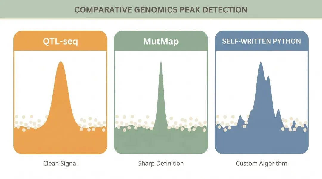
我自己用同一组水稻数据跑过 3 个工具,结果对比如下:
六、我的工具组合策略
跑 BSA 项目,我会双工具交叉验证:
6.1 主力:QTL-seqr
跑主体分析 出主图 审稿人接受度最高
6.2 辅助:自写 Python
上篇的脚本 用于特殊场景(如自定阈值、自定统计量) 跟 QTL-seqr 交叉验证主峰位置
6.3 备选:MutMap
如果数据是 EMS 诱变 如果走 MutMap 路线
6.4 探索:DeepBSA
池太小(< 20 株/池)才用 探索性分析 不当主图
七、软件安装 5 个常见问题
7.1 QTLseqr 装不上
报错 package 'xxx' is not available:
ounter(lineounter(line# 装依赖install.packages(c("dplyr", "ggplot2", "vcfR", "tidyr", "data.table"))
7.2 cyvcf2 装不上(Python)
ounter(lineounter(line# conda 装最稳mamba install -c bioconda cyvcf2
7.3 DeepBSA 缺 GPU
DeepBSA 默认用 GPU,没 GPU 也能跑(CPU 模式),但慢 20 倍。CPU 模式:
ounter(linepython DeepBSA.py --device cpu ...
7.4 VCF 读不了
ounter(lineounter(lineounter(lineounter(line# 常见原因:VCF 没压缩索引# 用 bcftools 处理bcftools view -Oz file.vcf > file.vcf.gzbcftools index file.vcf.gz
7.5 中文路径报错
R 跟 Python 都不喜欢 Windows 中文路径。把你的 BSA 项目放在纯英文路径。
八、自检 Checklist
[ ] 工具装了,import 正常? [ ] VCF 能被工具读取? [ ] 池样本名匹配? [ ] 至少跑出 1 张 Manhattan 图? [ ] 至少 1 个主峰超过阈值? [ ] 候选区间 < 10 Mb?
下篇预告
下一篇是从区间到基因——拿到候选区间后怎么注释、怎么 GO/KEGG 富集、怎么找候选基因。这步是从"定位"到"解释生物学"的跨越。
一句话总结
BSA 工具选择的精髓:QTL-seqr 当主力 + 自写 Python 当备胎 + MutMap 走突变路线。三个工具的图互相印证,比任何单一工具都稳。
你跑过哪个 BSA 工具?结果怎么样?评论区聊聊 👇