 夜雨聆风
夜雨聆风代码实战 | 下载 ERA5 并计算 GPI(台风最大潜在强度)
前言
如何计算 GPI 在之前的 skyborn 库有介绍,之前的示例对于 era5 的变量名有小小的瑕疵。
本期文章给出一份"开箱即用"的完整脚本,实现功能如下:
自动从 CDS(Copernicus Data Store)下载 ERA5 单层/多层变量; 把下载好的文件拼接成一场台风研究常用的 0.25°、逐小时或逐日数据; 用 Skyborn(xarray 接口)一次性算出整个区域/时段的台风最大潜在强度(PI)。
脚本已经在 Linux / macOS / Win 上 Python≥3.9 实测通过,只需把 dates、area 改成自己需要的时间段/区域即可直接跑。
0. 环境准备
# 建议先建个干净环境conda create -n era5_PI python=3.11 -yconda activate era5_PI# 一次性装好pip install cdsapi skyborn xarray netcdf4 dask1. 在 CDS 注册并获取 API key
注册 https://cds.climate.copernicus.eu/ 登录后右上角 "My API key" -> 复制两行 url+key 写入本地文件 ~/.cdsapirc(Win 用户路径为%USERPROFILE%\.cdsapirc)
url: https://cds.climate.copernicus.eu/api/v2key: 你的uid:你的key2. 下载脚本:get_era5_for_PI.py
#!/usr/bin/env python"""一键下载 ERA5 计算台风 PI 所需变量单层:sst, msl多层:t, q (37 层,1000 → 1 hPa,Skyborn 官方推荐)运行前请先在 ~/.cdsapirc 里放好 CDS API key"""import os, cdsapi, datetime as dtfrom pathlib import Path# ---------------- 用户区域 ----------------dates = ["2023-08-01/to/2023-08-31"] # 可写多段area = [30, 110, 15, 140] # N/W/S/Eoutdir = Path("ERA5")# -----------------------------------------outdir.mkdir(exist_ok=True)c = cdsapi.Client()# 单层single = ['sea_surface_temperature', 'mean_sea_level_pressure']c.retrieve("reanalysis-era5-single-levels", {"product_type": "reanalysis","variable" : single,"date" : dates,"area" : area,"grid" : "0.25/0.25","format" : "netcdf","time" : "00/to/23/by/1", # 逐小时;如只需日平均改成 ["00:00", "12:00"] }, outdir / "ERA5_single.nc")# 多层levels = [1000, 975, 950, 925, 900, 875, 850, 825, 800, 775, 750, 700,650, 600, 550, 500, 450, 400, 350, 300, 250, 200,175, 150, 125, 100, 70, 50, 30, 20, 10, 7, 5, 3, 2, 1]multi = ['temperature', 'specific_humidity']c.retrieve("reanalysis-era5-pressure-levels", {"product_type" : "reanalysis","variable" : multi,"pressure_level" : levels,"date" : dates,"area" : area,"grid" : "0.25/0.25","format" : "netcdf","time" : "00/to/23/by/1", }, outdir / "ERA5_multilevel.nc")print("✅ 下载完成!文件位于", outdir.absolute())运行
python get_era5_for_PI.py即可得到
ERA5/ ├─ ERA5_single.nc └─ ERA5_multilevel.nc3. 计算脚本:calc_PI_ERA5.py
#!/usr/bin/env python"""用 Skyborn 计算 ERA5 的台风最大潜在强度 PI支持 1D/3D/4D 场,自动识别单位 & 缺测"""import xarray as xrfrom skyborn.calc.GPI.xarray import potential_intensity# ---------------- 读数据 -----------------ds_s = xr.open_dataset("/home/mw/input/gpi4714/ERA5_single.nc")ds_m = xr.open_dataset("/home/mw/input/gpi4714/ERA5_multilevel.nc")# 如果下载的是逐小时,但只想做日平均,可 resample# ds_s = ds_s.resample(time='1D').mean()# ds_m = ds_m.resample(time='1D').mean()# 确保单位属性(ERA5 本来就有,保险起见再写一次)ds_s['sst'].attrs['units'] = 'K'ds_s['msl'].attrs['units'] = 'Pa'ds_m['t'].attrs['units'] = 'K'ds_m['q'].attrs['units'] = 'kg kg-1'# 混合比/比湿# 可选:只挑热带海域(SST≥26.5°C)mask = ds_s['sst'] >= 299.65# 26.5°Csst = ds_s['sst'].where(mask)msl = ds_s['msl'].where(mask)# 多层变量也做同样掩膜t = ds_m['t'].where(mask)q = ds_m['q'].where(mask)# ---------------- 计算 PI ---------------print("🌀 开始计算 Potential Intensity ...")pi_ds = potential_intensity( sst = sst, psl = msl, pressure_levels = ds_m['pressure_level'], temperature = t, mixing_ratio = q)# ---------------- 保存 -----------------outfile = "ERA5_PI_aug2023.nc"pi_ds.to_netcdf(outfile)print(f"✅ 计算完成!结果已写入 {outfile}")输出示例:
🌀 开始计算 Potential Intensity ...Missing values detected in: SST(NaN), PSL(NaN), temperature(NaN), mixing_ratio(NaN). Using missing value handling version.✅ 计算完成!结果已写入 ERA5_PI_aug2023.nc计算结果可视化示例:
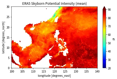
快速可视化:
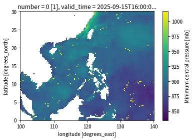
import matplotlib.pyplot as pltpi_ds = xr.open_dataset("ERA5_PI_aug2023.nc")pi_ds['pi'].mean('valid_time').plot(cmap='jet', vmin=20, vmax=90)plt.title("ERA5 Skyborn Potential Intensity (mean)")plt.tight_layout()plt.show()查看最小气压:
pi_ds.min_pressure[16].plot()最小气压分布示例:
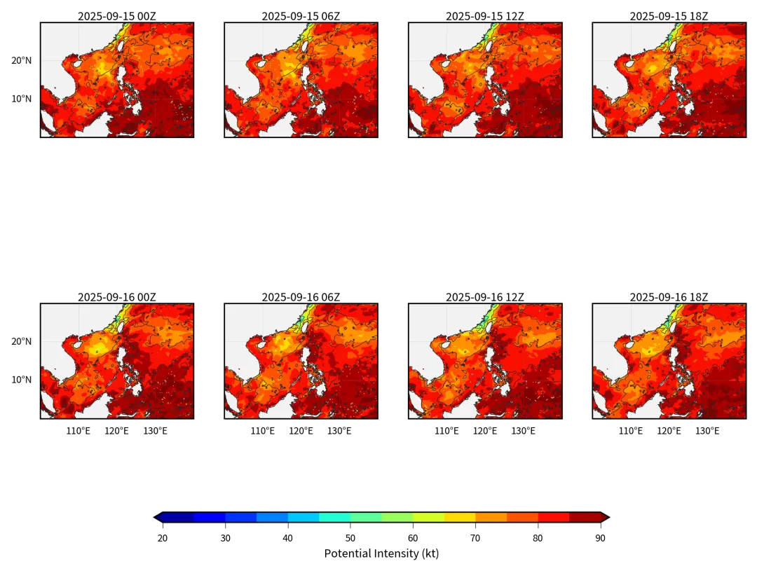
4. 细化绘图
import xarray as xrimport matplotlib.pyplot as pltimport matplotlib.ticker as mtickerimport cartopy.crs as ccrsimport cartopy.feature as cfeatureimport numpy as npimport matplotlib.patches as mpatchesfrom matplotlib.colors import ListedColormapimport osimport cmaps# ------------------------------------------------------# 1. 数据# ------------------------------------------------------ds = xr.open_dataset('ERA5_PI_aug2023.nc')pi = ds['pi'] # (48, 121, 161)sel = pi.valid_time.dt.hour.isin([0, 6, 12, 18])pi = pi.sel(valid_time=sel) # 8 个时刻pmin = ds['min_pressure'].sel(valid_time=pi.valid_time)# ------------------------------------------------------# 2. 颜色表# ------------------------------------------------------cmap = 'jet'levels = np.arange(20, 91, 5)norm = plt.Normalize(20, 90)# ------------------------------------------------------# 3. 底图函数# ------------------------------------------------------defadd_geo(ax, left=False, bottom=False): ax.set_extent([100, 140, 0, 30], crs=ccrs.PlateCarree()) ax.add_feature(cfeature.LAND.with_scale('50m'), facecolor=[.95, .95, .95], edgecolor='none', zorder=1) ax.add_feature(cfeature.COASTLINE.with_scale('50m'), linewidth=.4, edgecolor='0.15', zorder=2) gl = ax.gridlines(draw_labels=True, linewidth=.15, color='gray', alpha=.4, linestyle='-', zorder=3) gl.top_labels = gl.right_labels = False gl.left_labels = left gl.bottom_labels= bottom gl.xlocator = mticker.FixedLocator(np.arange(100, 141, 10)) gl.ylocator = mticker.FixedLocator(np.arange(0, 31, 10)) gl.xlabel_style = {'fontsize': 6} gl.ylabel_style = {'fontsize': 6}# ------------------------------------------------------# 4. 画布# ------------------------------------------------------fig = plt.figure(figsize=(8,6), dpi=300) # 180 mm 宽axes = []for i in range(8): left = (i % 4 == 0) # 最左列 bottom= (i // 4 == 1) # 最下行 ax = fig.add_subplot(2, 4, i+1, projection=ccrs.PlateCarree()) add_geo(ax, left=left, bottom=bottom) axes.append(ax)# ------------------------------------------------------# 5. 绘图# ------------------------------------------------------for ax, t in zip(axes, pi.valid_time): pi_t = pi.sel(valid_time=t) pm_t = pmin.isel(valid_time=i) cf = ax.contourf(pi_t.longitude, pi_t.latitude, pi_t, levels=levels, cmap=cmap, norm=norm, extend='both', transform=ccrs.PlateCarree(), zorder=1) cs = ax.contour(pm_t.longitude, pm_t.latitude, pm_t, levels=6, colors='0.15', linewidths=.3, transform=ccrs.PlateCarree(), zorder=2) ax.set_title(t.dt.strftime('%Y-%m-%d %HZ').values, size=7, pad=1)# ------------------------------------------------------# 6. colorbar# ------------------------------------------------------cbar_ax = fig.add_axes([0.25, 0.06, 0.5, 0.015])cbar = fig.colorbar(cf, cax=cbar_ax, orientation='horizontal', extend='both', extendfrac=0.02, ticks=levels[::2])cbar.ax.set_xlabel('Potential Intensity (kt)', fontsize=7, labelpad=3)cbar.ax.tick_params(labelsize=6, width=.3)# ------------------------------------------------------# 7. 保存# ------------------------------------------------------# plt.subplots_adjust(left=0.04, right=0.96, top=0.94, bottom=0.12,# hspace=0.02, wspace=0.06)plt.show()# plt.savefig('fig_pi_8panel.pdf', dpi=300, bbox_inches='tight')# plt.close()细化绘图示例(8 面板图):
5. 常见坑提醒
垂直层太少 → PI 偏低:至少 15 层,最好 30+ 层;上面下载的 37 层足够。 把 RH 直接当 q 用 → 结果全错,ERA5 的 q就是混合比,无需换算。单位属性缺失 → Skyborn 不会自动识别,脚本里已补写。 内存爆掉:全球 0.25°× 逐小时 ×37 层非常庞大,建议先裁剪区域/时段,或分块 dask。
这样,从"零"到拿到一张漂亮的台风潜在强度图, 全程只需要两条命令:
python get_era5_for_PI.py # 下载python calc_PI_ERA5.py # 计算快去试试吧!祝科研顺利 🌪️


微信公号:Earth-Ai
商务联系:Earth_Ai
