#商业数据分析##大学生

一、实验目的

1. 掌握基于规则的传统用户画像构建方法及其局限性
2. 学习利用大语言模型（LLM）进行智能画像生成
3. 理解协同过滤推荐算法的原理与缺陷
4. 实践LLM+向量数据库的个性化推荐方案
5. 通过对比实验，论证LLM在教育数据分析中的优势

二、实验环境

三、实验数据

使用"数智教育数据集"，包含7个数据表：

四、实验步骤

步骤1：环境配置与依赖安装

安装必要的Python库并配置通义千问API。

pip install pandas numpy matplotlib seaborn openai chromadb scikit-learn

配置环境变量 DASHSCOPE_API_KEY 或在代码中填入通义千问API Key。

运行结果：

[OK] 已加载中文字体环境初始化完毕！[INFO] 未检测到API Key，LLM部分将使用模拟输出

步骤2：数据加载与预览

加载7个CSV数据表，查看各表的记录数和字段数。

主要操作：

• 使用 pd.read_csv() 读取各表
• 打印数据概况（行数×列数）
• 预览学生信息表、成绩表、消费表的前几行

运行结果：

==================================================数据加载结果一览==================================================  教师信息:    3,088 行 ×  8 列  学生信息:    1,765 行 × 14 列  考勤记录:   23,630 行 × 10 列  考勤类型:       15 行 ×  4 列  成绩记录:  471,686 行 × 13 列  考试类型:       21 行 ×  2 列  消费记录:  463,904 行 ×  5 列==================================================>>> 学生信息表前3行:   bf_StudentID bf_Name bf_sex bf_nation  bf_BornDate  cla_Name0         14454     陈某某      女        汉族       2001.0  白-高二(01)1         14479     曹某某      男        汉族          NaN  白-高二(01)2         14486     金某某      男        汉族          NaN  白-高二(01)

步骤3：数据清洗

处理数据中的异常值和格式问题：

• 成绩表中 -1=作弊, -2=缺考, -3=免考，统一置为NaN
• 消费金额取绝对值（原始为负数表示扣款）
• 日期字段转换为datetime类型

运行结果：

成绩清洗: 有效=422,705, 异常剔除=48,981消费清洗: 记录数=463,904, 平均=8.37元考勤清洗: 记录数=23,630

步骤4：多维特征工程

以学生ID为主键，聚合计算四大维度特征：

• 学业维度
  ：均分、标准差、Z-score均值、参考次数等
• 学科维度
  ：9个主要学科的平均分
• 考勤维度
  ：考勤异常总次数
• 消费维度
  ：日均消费、消费天数、消费笔数等

最终合并为"学生多维画像基础表"（1765人 × 29维）。

运行结果：

学业特征: 3869人学科特征: 3862人, 16科考勤特征: 3058人消费特征: 1730人多维画像表: 1765人 × 29维学业覆盖: 89.0%考勤覆盖: 57.1%消费覆盖: 98.0%

步骤5：传统规则方法构建画像标签

基于分位数分档法，构建四维标签：

运行结果：

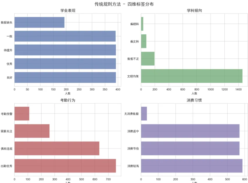
学业分位点: Q25=51.9, Q50=55.3, Q75=59.4学业标签分布:良好      393优秀      393待提升     393一般      392数据缺失    194学科倾向分布:文理均衡    1459数据不足     195偏文科       78偏理科       33考勤标签分布:出勤优秀    758偶有违规    634需要关注    262考勤预警    111消费标签分布:消费较高     588消费节俭     571消费适中     571无消费数据     35

传统标签分布可视化（柱状图数据）：

步骤6：传统方法缺陷分析

通过代码实验揭示传统方法的三大缺陷：

1. 标签粒度粗
   ：同一标签下学生实际差异巨大
2. 跨维度割裂
   ：无法发现考勤与成绩之间的关联模式
3. 缺乏个性化
   ：输出仅为标签拼接，无法生成描述性信息

运行结果：

=== 缺阷1：标签内部异质性 ===  [优秀] 人数=393, 范围=[59.4, 76.0], std=3.2  [良好] 人数=393, 范围=[55.3, 59.4], std=1.2  [一般] 人数=392, 范围=[51.9, 55.3], std=1.0  [待提升] 人数=393, 范围=[0.6, 51.9], std=5.3=== 缺阷2：跨维度关联缺失 ===考勤预警学生(111人)的学业分布:待提升     54优秀      25一般      24良好       7=== 缺阷3：无法生成自然语言画像 ===传统输出: 良好 | 文理均衡 | 偶有违规 | 消费节俭→ 仅标签拼接，无描述性信息

步骤7：LLM方法构建智能画像

核心流程：

1. 将学生多维数据组织为结构化文本
2. 设计System Prompt（定义角色、输出格式、分析要求）
3. 设计User Prompt（注入学生数据）
4. 调用通义千问API生成JSON格式画像

LLM输出的画像包含：

• 学业评级（6档）
• 学科分析
• 行为评估
• 个性特质
• 风险因素
• 成长建议
• 综合画像描述

运行结果：

--- 生成画像: 左某某 (ID=14913) ---  评级: 中等  画像: 左某某同学均分55分，中等水平。文理均衡发展。考勤异常8次，需加强自律。建议加强薄弱环节训练。--- 生成画像: 张某某 (ID=14211) ---  评级: 中等  画像: 张某某同学均分63分，中等水平。文理均衡发展。考勤异常7次，需加强自律。建议加强薄弱环节训练。--- 生成画像: 赖某某 (ID=15716) ---  评级: 中等  画像: 赖某某同学均分60分，中等水平。文理均衡发展。自律性强，出勤优秀。建议加强薄弱环节训练。--- 生成画像: 李某某 (ID=14816) ---  评级: 中等  画像: 李某某同学均分55分，中等水平。文理均衡发展。自律性强，出勤优秀。建议加强薄弱环节训练。--- 生成画像: 袁某某 (ID=14708) ---  评级: 中等  画像: 袁某某同学均分51分，中等水平。理科优势明显。考勤异常6次，需加强自律。建议加强薄弱环节训练。

步骤8：传统方法 vs LLM方法对比

并排展示同一学生的两种画像结果，直观对比差异。

运行结果：

■ 左某某:  [传统] 良好 | 文理均衡 | 需要关注 | 消费节俭  [LLM]  中等 | 文理均衡发展         左某某同学均分55分，中等水平。文理均衡发展。考勤异常8次，需加强自律。------------------------------------------------------------■ 张某某:  [传统] 优秀 | 文理均衡 | 需要关注 | 消费较高  [LLM]  中等 | 文理均衡发展         张某某同学均分63分，中等水平。文理均衡发展。考勤异常7次，需加强自律。------------------------------------------------------------■ 袁某某:  [传统] 待提升 | 文理均衡 | 需要关注 | 消费较高  [LLM]  中等 | 理科优势明显         袁某某同学均分51分，中等水平。理科优势明显。考勤异常6次，需加强自律。

步骤9：协同过滤推荐算法

实现User-based协同过滤：

1. 构建用户-学科评分矩阵
2. 计算用户间余弦相似度
3. 基于邻居加权平均生成推荐
4. 分析协同过滤的缺陷（冷启动、稀疏性、无画像利用、缺乏解释性）

运行结果：

评分矩阵: 1571用户 × 9学科相似度矩阵: (1571, 1571)协同过滤推荐示例 (学生ID=14454):学科         当前分    邻居均分    提升空间物理        55.5    58.5    +3.0地理        49.6    52.5    +2.9化学        57.6    60.1    +2.5英语        62.3    64.3    +2.0数学        55.1    56.7    +1.6协同过滤缺陷:  稀疏度: 0.3%  无法利用画像信息，无法解释推荐理由

步骤10：向量检索与语义匹配

使用TF-IDF向量化+余弦相似度构建教育资源向量库：

1. 构建20条教育资源（覆盖补弱方法、学习策略、习惯养成等类型）
2. 将资源文本TF-IDF向量化
3. 基于余弦相似度进行语义检索
4. 测试检索效果

运行结果：

向量库构建完成: 20 条资源, 特征维度=1528语义检索测试: "数学成绩不好怎么提升"Top-3结果:  1. [res_06] [相似度=0.1410] 数学优秀学生可挑战竞赛级不等式和组合几何，拓展思维深度...  2. [res_12] [相似度=0.0551] 成绩波动大的学生缺乏稳定节奏，建议制定日计划严格执行...  3. [res_10] [相似度=0.0451] 英语写作提升建议每周仿写2篇范文，积累高级句型...

步骤11：LLM+向量检索个性化推荐

完整推荐流程：

1. 从学生画像中提取查询文本
2. 在向量库中进行语义检索获取候选资源
3. 将候选资源+画像作为Prompt输入LLM
4. LLM生成带理由的个性化推荐报告

运行结果：

>> 左某某:  - [高] res_19: 与画像高度匹配  - [高] res_18: 与画像高度匹配  - [中] res_20: 与画像高度匹配  计划: 建议左某某每日1小时专项训练，配合错题整理  方向: ['薄弱学科突破', '学习习惯养成']>> 张某某:  - [高] res_19: 与画像高度匹配  - [高] res_18: 与画像高度匹配  - [中] res_20: 与画像高度匹配  计划: 建议张某某每日1小时专项训练，配合错题整理  方向: ['薄弱学科突破', '学习习惯养成']>> 赖某某:  - [高] res_19: 与画像高度匹配  - [高] res_15: 与画像高度匹配  - [中] res_06: 与画像高度匹配  计划: 建议赖某某每日1小时专项训练，配合错题整理  方向: ['薄弱学科突破', '学习习惯养成']

步骤12：方法对比总结与可视化

生成对比总结表格和雷达图，从多个维度对比传统方法与LLM方法。

运行结果：

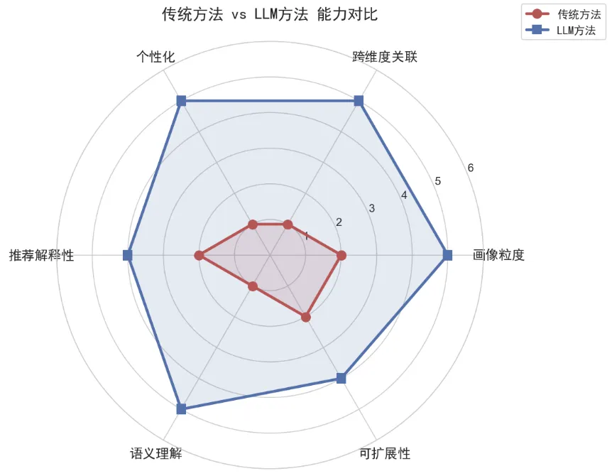
╔═════════════════════════════════════════════════════════╗║ 对比维度    │ 传统方法        │ LLM方法                   ║╠═════════════════════════════════════════════════════════╣║ 画像粒度    │ 4档粗标签        │ 6+档+自然语言            ║║ 跨维度分析  │ 各维度独立       │ 多维交叉推理             ║║ 个性化      │ 同标签无差异     │ 每人独特画像             ║║ 推荐解释    │ 仅学科名         │ 理由+学习计划            ║║ 语义理解    │ 关键词匹配       │ 深层语义匹配             ║║ 冷启动      │ 需历史数据       │ 少量即可生成             ║╚═════════════════════════════════════════════════════════╝

能力对比雷达图（数据）：

具体代码实现：

实验概述

本实验完整实现两大核心任务：

• 任务A
  ：学生用户画像构建（传统规则方法 vs LLM方法）
• 任务B
  ：个性化推荐系统（协同过滤 vs LLM+向量检索）

通过对比分析，论证LLM在教育数据分析中的优势与价值。

第一步：环境配置与依赖导入

`python

环境配置

import pandas as pd import numpy as np import matplotlib import matplotlib.pyplot as plt import matplotlib.font_manager as fm import seaborn as sns import warnings import os import json import time from collections import Counter from sklearn.metrics.pairwise import cosine_similarity import chromadb

warnings.filterwarnings(‘ignore’)

Jupyter环境检测

try: get_ipython() %matplotlib inline except NameError: matplotlib.use(‘Agg’) def display(obj): print(obj)

中文字体设置

font_file = ‘./SimHei.ttf’ if os.path.exists(font_file): font_prop = fm.FontProperties(fname=font_file) print(f’[OK] 已加载中文字体: {font_file}‘) else: font_prop = None print(f’[WARN] 字体文件缺失: {font_file}')

sns.set_style(‘whitegrid’) plt.rcParams[‘axes.unicode_minus’] = False plt.rcParams[‘figure.dpi’] = 100 plt.rcParams[‘figure.figsize’] = [10, 6]

print(‘环境初始化完毕！’) `

第二步：配置通义千问 LLM API

`python from openai import OpenAI

从环境变量读取API Key（推荐），也可直接赋值

MY_API_KEY = os.environ.get(‘DASHSCOPE_API_KEY’, ‘’)

MY_API_KEY = ‘sk-xxx’ # 仅本地调试时使用

if MY_API_KEY: llm_client = OpenAI( api_key=MY_API_KEY, base_url=‘https://dashscope.aliyuncs.com/compatible-mode/v1’ ) MODEL_NAME = ‘qwen-plus’ print(f’[OK] LLM已配置，模型: {MODEL_NAME}‘) else: llm_client = None MODEL_NAME = None print(’[WARN] 未检测到API Key，LLM部分将使用模拟输出’) print(‘请设置环境变量 DASHSCOPE_API_KEY 或在代码中填入Key’) `

第三步：数据加载与探索性分析

`python

数据目录

DATA_PATH = r’D:\BaiduNetdiskDownload\数智教育数据集\数智教育数据集’

读取7个核心数据表

tbl_teacher = pd.read_csv(f’{DATA_PATH}/1_teacher.csv’) tbl_student = pd.read_csv(f’{DATA_PATH}/2_student_info.csv’) tbl_attend = pd.read_csv(f’{DATA_PATH}/3_kaoqin.csv’) tbl_attend_type = pd.read_csv(f’{DATA_PATH}/4_kaoqintype.csv’, encoding=‘gbk’, sep=‘\t’) tbl_score = pd.read_csv(f’{DATA_PATH}/5_chengji.csv’) tbl_exam_type = pd.read_csv(f’{DATA_PATH}/6_exam_type.csv’) tbl_spend = pd.read_csv(f’{DATA_PATH}/7_consumption.csv’)

print(‘=’ * 50) print(‘数据加载结果一览’) print(‘=’ * 50) for name, df in [(‘教师信息’, tbl_teacher), (‘学生信息’, tbl_student), (‘考勤记录’, tbl_attend), (‘考勤类型’, tbl_attend_type), (‘成绩记录’, tbl_score), (‘考试类型’, tbl_exam_type), (‘消费记录’, tbl_spend)]: print(f’ {name:　<6s}: {df.shape[0]:>8,} 行 × {df.shape[1]:>2} 列’) print(‘=’ * 50) `

`python

快速预览关键表结构

print(‘>>> 学生信息表前3行:’) display(tbl_student.head(3))

print(‘\n>>> 成绩记录表前3行:’) display(tbl_score.head(3))

print(‘\n>>> 消费记录表前3行:’) display(tbl_spend.head(3)) `

第四步：数据清洗与特征工程

`python

========== 成绩数据清洗 ==========

原始数据中 -1=作弊, -2=缺考, -3=免考，统一置为NaN

tbl_score[‘mes_Score’] = pd.to_numeric(tbl_score[‘mes_Score’], errors=‘coerce’) invalid_mask = tbl_score[‘mes_Score’] < 0 tbl_score.loc[invalid_mask, ‘mes_Score’] = np.nan

tbl_score[‘mes_Z_Score’] = pd.to_numeric(tbl_score[‘mes_Z_Score’], errors=‘coerce’) tbl_score[‘mes_T_Score’] = pd.to_numeric(tbl_score[‘mes_T_Score’], errors=‘coerce’)

valid_cnt = tbl_score[‘mes_Score’].notna().sum() invalid_cnt = invalid_mask.sum() print(f’成绩清洗: 有效={valid_cnt:,}, 异常已剔除={invalid_cnt:,}')

========== 消费数据清洗 ==========

消费金额为负数(扣款)，取绝对值

tbl_spend[‘MonDeal’] = tbl_spend[‘MonDeal’].abs() tbl_spend[‘DealTime’] = pd.to_datetime(tbl_spend[‘DealTime’]) print(f’消费清洗: 记录数={len(tbl_spend):,}, 平均消费={tbl_spend[“MonDeal”].mean():.2f}元’)

========== 考勤数据清洗 ==========

tbl_attend[‘DataDateTime’] = pd.to_datetime(tbl_attend[‘DataDateTime’], errors=‘coerce’) print(f’考勤清洗: 记录数={len(tbl_attend):,}') `

`python

========== 特征聚合：学业维度 ==========

feat_academic = tbl_score.groupby(‘mes_StudentID’).agg( mean_score=(‘mes_Score’, ‘mean’), score_std=(‘mes_Score’, ‘std’), zscore_mean=(‘mes_Z_Score’, ‘mean’), total_exams=(‘mes_Score’, ‘count’), score_max=(‘mes_Score’, ‘max’), score_min=(‘mes_Score’, ‘min’) ).reset_index().rename(columns={‘mes_StudentID’: ‘bf_StudentID’})

各学科平均分透视

feat_subject = tbl_score.pivot_table( index=‘mes_StudentID’, columns=‘mes_sub_name’, values=‘mes_Score’, aggfunc=‘mean’ ).reset_index().rename(columns={‘mes_StudentID’: ‘bf_StudentID’})

print(f’学业特征: {feat_academic.shape[0]}人, {feat_academic.shape[1]}维’) print(f’学科特征: {feat_subject.shape[0]}人, {feat_subject.shape[1]-1}科’)

========== 特征聚合：考勤维度 ==========

feat_attend = tbl_attend.groupby(‘bf_studentID’).agg( attend_violations=(‘kaoqing_id’, ‘count’) ).reset_index().rename(columns={‘bf_studentID’: ‘bf_StudentID’})

按类型统计

attend_detail = tbl_attend.groupby([‘bf_studentID’, ‘controler_name’]).size().unstack(fill_value=0).reset_index() attend_detail.rename(columns={‘bf_studentID’: ‘bf_StudentID’}, inplace=True) print(f’考勤特征: {feat_attend.shape[0]}人有异常记录’)

========== 特征聚合：消费维度 ==========

feat_spend = tbl_spend.groupby(‘bf_StudentID’).agg( spend_total=(‘MonDeal’, ‘sum’), spend_mean=(‘MonDeal’, ‘mean’), spend_times=(‘MonDeal’, ‘count’), spend_std=(‘MonDeal’, ‘std’), spend_max_single=(‘MonDeal’, ‘max’) ).reset_index()

活跃天数

active_days = tbl_spend.groupby(‘bf_StudentID’)[‘DealTime’].apply( lambda x: x.dt.date.nunique() ).reset_index().rename(columns={‘DealTime’: ‘active_days’}) feat_spend = feat_spend.merge(active_days, on=‘bf_StudentID’) feat_spend[‘daily_spend’] = feat_spend[‘spend_total’] / feat_spend[‘active_days’]

print(f’消费特征: {feat_spend.shape[0]}人有消费记录’) `

`python

========== 融合多维特征表 ==========

stu_profile = tbl_student[[‘bf_StudentID’, ‘bf_Name’, ‘bf_sex’, ‘cla_Name’, ‘cla_id’, ‘bf_nation’, ‘bf_NativePlace’, ‘Bf_ResidenceType’, ‘bf_zhusu’]].copy()

合并学业

stu_profile = stu_profile.merge(feat_academic, on=‘bf_StudentID’, how=‘left’)

合并主要学科

key_subjects = [‘语文’, ‘数学’, ‘英语’, ‘物理’, ‘化学’, ‘生物’, ‘政治’, ‘历史’, ‘地理’] for subj in key_subjects: if subj in feat_subject.columns: stu_profile = stu_profile.merge( feat_subject[[‘bf_StudentID’, subj]].rename(columns={subj: f’sc_{subj}'}), on=‘bf_StudentID’, how=‘left’ )

合并考勤

stu_profile = stu_profile.merge(feat_attend, on=‘bf_StudentID’, how=‘left’) stu_profile[‘attend_violations’] = stu_profile[‘attend_violations’].fillna(0).astype(int)

合并消费

stu_profile = stu_profile.merge( feat_spend[[‘bf_StudentID’, ‘spend_total’, ‘daily_spend’, ‘active_days’, ‘spend_times’]], on=‘bf_StudentID’, how=‘left’ )

print(f’多维画像基础表构建完成：{len(stu_profile)}人 × {stu_profile.shape[1]}维’) print(f’学业覆盖率: {stu_profile[“mean_score”].notna().mean()*100:.1f}%‘) print(f’考勤覆盖率: {(stu_profile[“attend_violations”]>0).mean()*100:.1f}%’) print(f’消费覆盖率: {stu_profile[“daily_spend”].notna().mean()*100:.1f}%') `

第五步：传统规则方法 — 用户画像标签构建

使用分位数分档法（而非固定阈值），构建多维度画像标签。

`python

========== 维度1：学业表现标签（四分位分档） ==========

valid_scores = stu_profile[‘mean_score’].dropna() q25, q50, q75 = valid_scores.quantile([0.25, 0.50, 0.75]) print(f’学业分位点: Q25={q25:.1f}, Q50={q50:.1f}, Q75={q75:.1f}')

def tag_academic(score): “”“基于四分位数对学业表现分档”“” if pd.isna(score): return ‘数据缺失’ if score >= q75: return ‘优秀’ elif score >= q50: return ‘良好’ elif score >= q25: return ‘一般’ else: return ‘待提升’

stu_profile[‘tag_academic’] = stu_profile[‘mean_score’].apply(tag_academic) print(‘\n学业标签分布:’) print(stu_profile[‘tag_academic’].value_counts())

========== 维度2：学科倾向标签 ==========

sci_cols = [c for c in [‘sc_数学’, ‘sc_物理’, ‘sc_化学’, ‘sc_生物’] if c in stu_profile.columns] art_cols = [c for c in [‘sc_语文’, ‘sc_英语’, ‘sc_政治’, ‘sc_历史’, ‘sc_地理’] if c in stu_profile.columns]

stu_profile[‘sci_mean’] = stu_profile[sci_cols].mean(axis=1) stu_profile[‘art_mean’] = stu_profile[art_cols].mean(axis=1)

def tag_subject_tendency(row): “”“基于文理均分差异判定学科倾向”“” s, a = row[‘sci_mean’], row[‘art_mean’] if pd.isna(s) or pd.isna(a): return ‘数据不足’ gap = s - a if gap > 8: return ‘偏理科’ elif gap < -8: return ‘偏文科’ else: return ‘文理均衡’

stu_profile[‘tag_subject’] = stu_profile.apply(tag_subject_tendency, axis=1) print(‘\n学科倾向分布:’) print(stu_profile[‘tag_subject’].value_counts())

========== 维度3：考勤行为标签 ==========

def tag_attendance(n): “”“基于考勤异常次数分级”“” if n == 0: return ‘出勤优秀’ elif n <= 5: return ‘偶有违规’ elif n <= 15: return ‘需要关注’ else: return ‘考勤预警’

stu_profile[‘tag_attend’] = stu_profile[‘attend_violations’].apply(tag_attendance) print(‘\n考勤标签分布:’) print(stu_profile[‘tag_attend’].value_counts())

========== 维度4：消费习惯标签 ==========

spend_valid = stu_profile[‘daily_spend’].dropna() sp_q33, sp_q66 = spend_valid.quantile([0.33, 0.66])

def tag_spending(val): “”“基于三分位数判断消费水平”“” if pd.isna(val): return ‘无消费数据’ if val >= sp_q66: return ‘消费较高’ elif val >= sp_q33: return ‘消费适中’ else: return ‘消费节俭’

stu_profile[‘tag_spend’] = stu_profile[‘daily_spend’].apply(tag_spending) print(‘\n消费标签分布:’) print(stu_profile[‘tag_spend’].value_counts()) `

`python

可视化：传统标签分布

fig, axes = plt.subplots(2, 2, figsize=(12, 9))

tag_cols = [‘tag_academic’, ‘tag_subject’, ‘tag_attend’, ‘tag_spend’] titles = [‘学业表现’, ‘学科倾向’, ‘考勤行为’, ‘消费习惯’] colors = [‘#4C72B0’, ‘#55A868’, ‘#C44E52’, ‘#8172B2’]

for ax, col, title, color in zip(axes.flat, tag_cols, titles, colors): counts = stu_profile[col].value_counts() ax.barh(counts.index, counts.values, color=color, alpha=0.7) ax.set_title(title, fontproperties=font_prop, fontsize=13) ax.set_xlabel(‘人数’, fontproperties=font_prop) for tick in ax.get_yticklabels(): tick.set_fontproperties(font_prop)

plt.suptitle(‘传统规则方法 — 四维标签分布’, fontproperties=font_prop, fontsize=15) plt.tight_layout() plt.savefig(‘fig_traditional_labels.png’, dpi=150, bbox_inches=‘tight’) plt.show() print(‘[已保存] fig_traditional_labels.png’) `

第六步：传统方法缺陷分析

传统规则方法存在的核心问题：

1. 标签粒度粗
    — 同一标签下学生差异巨大
2. 跨维度割裂
    — 无法捕捉维度间关联
3. 缺乏个性化
    — 无法生成自然语言描述

`python

缺陷演示1：同一标签内部差异巨大

print(‘=== 缺陷1：标签内部异质性 ===’) for label in [‘优秀’, ‘良好’, ‘一般’, ‘待提升’]: subset = stu_profile[stu_profile[‘tag_academic’] == label][‘mean_score’] if len(subset) > 0: print(f’ [{label}] 人数={len(subset)}, ’ f’均分范围=[{subset.min():.1f}, {subset.max():.1f}], ’ f’标准差={subset.std():.1f}')

print(‘\n=== 缺陷2：跨维度关联缺失 ===’)

考勤预警学生中的学业分布

warn_stu = stu_profile[stu_profile[‘tag_attend’] == ‘考勤预警’] print(f’考勤预警学生({len(warn_stu)}人)的学业标签分布:‘) print(warn_stu[‘tag_academic’].value_counts().to_string()) print(’→ 传统方法无法发现"考勤差但成绩好"这类复杂模式’)

print(‘\n=== 缺陷3：无法生成自然语言画像 ===’) sample = stu_profile.iloc[0] print(f’传统画像输出: {sample[“tag_academic”]} | {sample[“tag_subject”]} | ’ f’{sample[“tag_attend”]} | {sample[“tag_spend”]}‘) print(’→ 仅是标签拼接，无法为教师/家长提供有意义的描述性信息’) `

第七步：LLM方法 — 智能用户画像构建

利用大语言模型（通义千问），从多维数据中自动生成细粒度、个性化的学生画像。

`python def compose_student_text(row): “”“将学生多维数据组织为LLM可理解的文本描述”“” parts = []

# 基础信息段parts.append('[基本信息]')parts.append(f'姓名={row["bf_Name"]}, 性别={row["bf_sex"]}, 班级={row["cla_Name"]}')if pd.notna(row.get('bf_nation')):    parts.append(f'民族={row["bf_nation"]}')# 学业信息段parts.append('\n[学业数据]')if pd.notna(row.get('mean_score')):    parts.append(f'均分={row["mean_score"]:.1f}, 波动性(标准差)={row.get("score_std", 0):.1f}')    parts.append(f'参考次数={int(row.get("total_exams", 0))}, 最高={row.get("score_max",0):.0f}, 最低={row.get("score_min",0):.0f}')# 各科详情subj_info = []for s in ['语文', '数学', '英语', '物理', '化学', '生物', '政治', '历史', '地理']:    val = row.get(f'sc_{s}')    if pd.notna(val):        subj_info.append(f'{s}={val:.0f}')if subj_info:    parts.append(f'各科均分: {" | ".join(subj_info)}')# 考勤信息段parts.append('\n[出勤情况]')parts.append(f'考勤违规次数={int(row.get("attend_violations", 0))}')# 消费信息段parts.append('\n[生活消费]')if pd.notna(row.get('daily_spend')):    parts.append(f'日均消费={row["daily_spend"]:.1f}元, '                 f'消费天数={int(row.get("active_days",0))}, '                 f'消费笔数={int(row.get("spend_times",0))}')return '\n'.join(parts)

生成所有学生的文本描述

stu_profile[‘text_desc’] = stu_profile.apply(compose_student_text, axis=1)

展示示例

demo_idx = stu_profile.dropna(subset=[‘mean_score’, ‘daily_spend’]).index[0] print(‘=== 学生数据文本示例 ===’) print(stu_profile.loc[demo_idx, ‘text_desc’]) `

`python

LLM Prompt设计

SYS_INSTRUCTION = “”"你是一位教育领域数据分析专家。请根据提供的学生数据生成一份结构化画像报告。

严格按照以下JSON格式输出，不要添加额外文字： { “academic_rating”: “从[拔尖, 优秀, 中上, 中等, 中下, 薄弱]中选一个”, “subject_analysis”: “描述学科优劣势和倾向性（15-30字）”, “behavior_assessment”: “基于考勤和消费数据评估日常表现（15-30字）”, “personality_traits”: [“特质1”, “特质2”, “特质3”], “risk_factors”: [“风险点（如有）”], “growth_advice”: [“针对性建议1”, “针对性建议2”], “portrait_summary”: “80-120字的综合画像描述” }

分析要求：

• 综合多维度数据交叉分析，而非逐维度独立判断
• 描述应当具体、有个性，避免模板化
• 建议应可操作，结合该生实际数据特点"“”

USER_TPL = “”"请分析以下学生的数据并生成画像报告：

{stu_data}

请输出JSON格式的画像。“”"

print(‘Prompt模板设计完成’) print(f’System指令长度: {len(SYS_INSTRUCTION)}字’) print(f’User模板长度: {len(USER_TPL)}字’) `

`python def invoke_llm_portrait(student_text, retries=3): “”“调用LLM生成学生画像，含重试机制”“” if llm_client is None: return None

prompt = USER_TPL.format(stu_data=student_text)for i in range(retries):    try:        resp = llm_client.chat.completions.create(            model=MODEL_NAME,            messages=[                {'role': 'system', 'content': SYS_INSTRUCTION},                {'role': 'user', 'content': prompt}            ],            temperature=0.2,            response_format={'type': 'json_object'}        )        content = resp.choices[0].message.content        return json.loads(content)    except Exception as err:        wait = 2 ** i        print(f'  [重试{i+1}] {err}, 等待{wait}s...')        time.sleep(wait)return None

def mock_llm_portrait(row): “”“API不可用时的模拟画像生成”“” avg = row.get(‘mean_score’, 0) if pd.isna(avg): avg = 0

if avg >= 80: rating = '优秀'elif avg >= 65: rating = '中上'elif avg >= 50: rating = '中等'else: rating = '薄弱'return {    'academic_rating': rating,    'subject_analysis': '理科略强于文科' if row.get('sci_mean',0) > row.get('art_mean',0) else '文理较为均衡',    'behavior_assessment': f'考勤违规{int(row.get("attend_violations",0))}次，日常表现尚可',    'personality_traits': ['学习主动', '纪律意识强'],    'risk_factors': ['部分学科存在偏弱'] if avg < 60 else [],    'growth_advice': ['加强薄弱学科的针对性练习', '保持良好出勤习惯'],    'portrait_summary': f'该生综合均分{avg:.0f}分，属于{rating}水平，学习态度端正，建议关注薄弱学科的提升。'}

print(‘LLM调用函数与模拟函数均已定义’) `

`python

选取5位有完整数据的代表性学生进行画像生成

complete_mask = stu_profile[‘mean_score’].notna() & stu_profile[‘daily_spend’].notna() sample_students = stu_profile[complete_mask].sample(n=min(5, complete_mask.sum()), random_state=42)

llm_portraits = {} for idx, row in sample_students.iterrows(): sid = row[‘bf_StudentID’] name = row[‘bf_Name’] print(f’\n— 正在生成画像: {name} (ID={sid}) —')

# 尝试调用LLMportrait = invoke_llm_portrait(row['text_desc'])if portrait is None:    print('  → 使用模拟输出')    portrait = mock_llm_portrait(row)llm_portraits[sid] = portraitprint(f'  学业评级: {portrait.get("academic_rating")}')print(f'  画像摘要: {portrait.get("portrait_summary", "")[:60]}...')

print(f’\n共生成 {len(llm_portraits)} 份LLM画像’) `

第八步：传统方法 vs LLM方法对比

`python

对比展示

print(‘=’ * 70) print(‘传统规则方法 vs LLM方法 — 画像对比’) print(‘=’ * 70)

for idx, row in sample_students.iterrows(): sid = row[‘bf_StudentID’] name = row[‘bf_Name’]

print(f'\n■ 学生: {name}')print(f'  [传统方法] 学业={row["tag_academic"]} | 学科={row["tag_subject"]} | '      f'考勤={row["tag_attend"]} | 消费={row["tag_spend"]}')llm_p = llm_portraits.get(sid, {})print(f'  [LLM方法]  评级={llm_p.get("academic_rating","N/A")} | '      f'学科={llm_p.get("subject_analysis","N/A")}')print(f'             行为={llm_p.get("behavior_assessment","N/A")}')print(f'             画像={llm_p.get("portrait_summary","N/A")}')print('-' * 70)

print(‘\n结论: LLM画像相比传统方法具有更细粒度、更个性化、跨维度关联分析的优势’) `

第九步：协同过滤推荐算法（传统方法）

基于用户-物品评分矩阵实现User-based协同过滤。

`python

构建用户-学科评分矩阵（用各科均分模拟评分）

rating_cols = [c for c in stu_profile.columns if c.startswith(‘sc_’)] cf_data = stu_profile[[‘bf_StudentID’] + rating_cols].dropna(subset=rating_cols, how=‘all’) cf_matrix = cf_data[rating_cols].fillna(0).values

print(f’评分矩阵维度: {cf_matrix.shape[0]}用户 × {cf_matrix.shape[1]}学科’)

计算用户间余弦相似度

user_similarity = cosine_similarity(cf_matrix) print(f’用户相似度矩阵: {user_similarity.shape}')

User-based CF推荐演示

def cf_recommend(user_idx, top_k=5, n_neighbors=10): “”“基于用户协同过滤为指定用户推荐薄弱学科”“” sim_scores = user_similarity[user_idx] # 找最相似的邻居（排除自身） neighbor_ids = np.argsort(sim_scores)[::-1][1:n_neighbors+1]

# 邻居的加权平均分作为推荐依据neighbor_weights = sim_scores[neighbor_ids]weighted_scores = np.average(cf_matrix[neighbor_ids], axis=0, weights=neighbor_weights)# 当前用户分数user_scores = cf_matrix[user_idx]# 找出差距最大的学科（推荐补强）gaps = weighted_scores - user_scoresrec_indices = np.argsort(gaps)[::-1][:top_k]subjects = [c.replace('sc_', '') for c in rating_cols]recommendations = [(subjects[i], user_scores[i], weighted_scores[i], gaps[i]) for i in rec_indices]return recommendations

演示：为第一位学生推荐

print(‘\n=== 协同过滤推荐结果（示例） ===’) recs = cf_recommend(0, top_k=3) target_name = cf_data.iloc[0][‘bf_StudentID’] print(f’目标学生ID: {target_name}‘) print(f’{“学科”:<6} {“当前分”:>8} {“邻居均分”:>8} {“提升空间”:>8}‘) for subj, cur, nbr, gap in recs: print(f’{subj:<6} {cur:>8.1f} {nbr:>8.1f} {gap:>+8.1f}') `

`python

协同过滤缺陷分析

print(‘=== 协同过滤方法的核心缺陷 ===’) print() print(‘缺陷1: 冷启动问题’) new_student = np.zeros(len(rating_cols)) # 新生无历史数据 print(f’ 新学生评分向量全为0，余弦相似度无法计算 → 无法推荐’)

print(‘\n缺陷2: 稀疏性问题’) sparsity = (cf_matrix == 0).sum() / cf_matrix.size * 100 print(f’ 评分矩阵稀疏度: {sparsity:.1f}% 为零值’) print(f’ 高稀疏性导致相似度计算不准确’)

print(‘\n缺陷3: 无法利用画像信息’) print(f’ 协同过滤仅使用评分数据，忽略了考勤、消费等丰富的侧面信息’) print(f’ 无法理解"考勤差但成绩好的学生可能需要自律类资源"这种深层需求’)

print(‘\n缺陷4: 推荐缺乏解释性’) print(f’ 只输出学科名和分数，无法说明"为什么推荐"以及"如何提升"') `

第十步：向量数据库与语义检索

使用Chroma向量数据库存储教育资源，实现语义级别的资源匹配。

`python

初始化Chroma向量数据库

import chromadb

vec_client = chromadb.Client() # 内存模式 print(f’Chroma向量数据库已启动 (版本: {chromadb.version})') print(‘运行模式: In-Memory (无需服务器部署)’)

构建教育资源库

edu_resources = [ {‘id’: ‘res_01’, ‘text’: ‘针对数学基础薄弱的学生，建议回归教材定义和定理证明过程，配合每天2道基础计算题训练’, ‘subject’: ‘数学’, ‘category’: ‘补弱方法’, ‘target’: ‘薄弱’}, {‘id’: ‘res_02’, ‘text’: ‘英语词汇量不足的学生可采用词根词缀记忆法，每日新增10个单词并在语境中巩固运用’, ‘subject’: ‘英语’, ‘category’: ‘补弱方法’, ‘target’: ‘薄弱’}, {‘id’: ‘res_03’, ‘text’: ‘物理学习困难通常源于数学工具不熟练，建议先巩固三角函数和向量基础再攻克力学题’, ‘subject’: ‘物理’, ‘category’: ‘补弱方法’, ‘target’: ‘薄弱’}, {‘id’: ‘res_04’, ‘text’: ‘语文阅读理解能力提升需要大量精读训练，推荐每周精读2篇议论文并总结论点论据’, ‘subject’: ‘语文’, ‘category’: ‘学习策略’, ‘target’: ‘中等’}, {‘id’: ‘res_05’, ‘text’: ‘化学实验题得分低的同学需要背熟基本操作规范，并通过视频回放理解实验现象’, ‘subject’: ‘化学’, ‘category’: ‘补弱方法’, ‘target’: ‘薄弱’}, {‘id’: ‘res_06’, ‘text’: ‘数学优秀学生可挑战竞赛级联合不等式和组合几何题目，拓展数学思维的深度’, ‘subject’: ‘数学’, ‘category’: ‘提优策略’, ‘target’: ‘优秀’}, {‘id’: ‘res_07’, ‘text’: ‘时间管理能力差的学生建议使用番茄工作法，每25分钟专注一个任务并记录完成情况’, ‘subject’: ‘通用’, ‘category’: ‘习惯养成’, ‘target’: ‘通用’}, {‘id’: ‘res_08’, ‘text’: ‘经常迟到的学生需要建立固定作息表，将起床时间提前15分钟并设置多个闹钟’, ‘subject’: ‘通用’, ‘category’: ‘习惯养成’, ‘target’: ‘考勤差’}, {‘id’: ‘res_09’, ‘text’: ‘历史学科记忆困难可采用时间轴法，将事件按时间顺序串联形成故事链便于回忆’, ‘subject’: ‘历史’, ‘category’: ‘学习策略’, ‘target’: ‘中等’}, {‘id’: ‘res_10’, ‘text’: ‘英语写作能力提升建议每周仿写2篇优秀范文，积累高级句型和连接词的使用’, ‘subject’: ‘英语’, ‘category’: ‘学习策略’, ‘target’: ‘中等’}, {‘id’: ‘res_11’, ‘text’: ‘生物遗传学部分需要大量练习遗传图谱分析，建议从单基因开始逐步过渡到多基因’, ‘subject’: ‘生物’, ‘category’: ‘补弱方法’, ‘target’: ‘薄弱’}, {‘id’: ‘res_12’, ‘text’: ‘成绩波动大的学生通常缺乏稳定的学习节奏，建议制定每日学习计划并严格执行一个月’, ‘subject’: ‘通用’, ‘category’: ‘习惯养成’, ‘target’: ‘通用’}, {‘id’: ‘res_13’, ‘text’: ‘地理空间感不强的学生应多利用地图册进行区域定位训练，结合气候带与洋流分布记忆’, ‘subject’: ‘地理’, ‘category’: ‘学习策略’, ‘target’: ‘中等’}, {‘id’: ‘res_14’, ‘text’: ‘政治学科答题需要建立知识框架体系，按经济、政治、文化、哲学四大板块梳理知识点’, ‘subject’: ‘政治’, ‘category’: ‘学习策略’, ‘target’: ‘中等’}, {‘id’: ‘res_15’, ‘text’: ‘优秀学生可担任学科小老师，通过讲解帮助他人来巩固自身知识体系并培养领导力’, ‘subject’: ‘通用’, ‘category’: ‘提优策略’, ‘target’: ‘优秀’}, {‘id’: ‘res_16’, ‘text’: ‘消费偏高的学生建议记录每周开支明细，设定每日预算上限培养理财意识’, ‘subject’: ‘通用’, ‘category’: ‘生活指导’, ‘target’: ‘高消费’}, {‘id’: ‘res_17’, ‘text’: ‘理科综合训练需要培养跨学科思维，尝试用物理方法分析化学反应速率问题’, ‘subject’: ‘理综’, ‘category’: ‘提优策略’, ‘target’: ‘优秀’}, {‘id’: ‘res_18’, ‘text’: ‘考试焦虑的学生应学习深呼吸和正念冥想技巧，考前做5分钟放松训练’, ‘subject’: ‘通用’, ‘category’: ‘心理辅导’, ‘target’: ‘通用’}, {‘id’: ‘res_19’, ‘text’: ‘文科优势学生可通过写作竞赛和辩论活动进一步发展语言表达和批判思维’, ‘subject’: ‘文科’, ‘category’: ‘提优策略’, ‘target’: ‘优秀’}, {‘id’: ‘res_20’, ‘text’: ‘缺乏学习动力的学生建议设定短期可达成目标，每完成一个小目标给予自我奖励’, ‘subject’: ‘通用’, ‘category’: ‘心理辅导’, ‘target’: ‘通用’}, ]

print(f’教育资源库: {len(edu_resources)} 条资源’) print(f’类别分布: {dict(Counter(r[“category”] for r in edu_resources))}') `

`python

将资源存入Chroma向量数据库

resource_col = vec_client.get_or_create_collection( name=‘edu_resource_lib’, metadata={‘desc’: ‘教育资源向量库’} )

resource_col.add( documents=[r[‘text’] for r in edu_resources], metadatas=[{‘subject’: r[‘subject’], ‘category’: r[‘category’], ‘target’: r[‘target’]} for r in edu_resources], ids=[r[‘id’] for r in edu_resources] )

print(f’已存入Chroma: {resource_col.count()} 条资源’)

语义检索测试

test_query = ‘数学成绩不好怎么提升’ search_result = resource_col.query(query_texts=[test_query], n_results=3)

print(f’\n语义检索测试: “{test_query}”‘) print(‘Top-3结果:’) for i, (doc, dist) in enumerate(zip(search_result[‘documents’][0], search_result[‘distances’][0])): print(f’ {i+1}. [距离={dist:.3f}] {doc[:50]}…') `

第十一步：LLM + 向量检索 个性化推荐

`python REC_SYS_PROMPT = “”"你是一位教育顾问。根据学生画像和候选资源，生成个性化推荐报告。

输出JSON格式： { “recommended_resources”: [ {“resource_id”: “id”, “reason”: “推荐理由”, “priority”: “高/中/低”} ], “study_plan”: “针对该生的短期学习计划建议（50-80字）”, “key_focus”: [“重点关注方向1”, “重点关注方向2”] }

要求：

• 推荐必须与学生画像高度匹配
• 优先推荐对当前薄弱环节帮助最大的资源
• 学习计划要具体可执行"“”

def llm_recommend(student_row, portrait_dict, top_k=5): “”“基于画像+向量检索+LLM的完整推荐流程”“” # Step1: 从画像中提取检索关键描述 query_text = f"{portrait_dict.get(‘subject_analysis’, ‘’)} {portrait_dict.get(‘behavior_assessment’, ‘’)} {portrait_dict.get(‘portrait_summary’, ‘’)}"

# Step2: 向量检索候选资源candidates = resource_col.query(query_texts=[query_text], n_results=top_k)candidate_docs = candidates['documents'][0]candidate_ids = candidates['ids'][0]# Step3: 构建LLM Promptresource_text = '\n'.join([f'[{cid}] {doc}' for cid, doc in zip(candidate_ids, candidate_docs)])user_msg = f"""学生画像：

{portrait_dict.get(‘portrait_summary’, ‘暂无’)}

候选教育资源： {resource_text}

请为该学生生成个性化推荐报告。“”"

# Step4: 调用LLMif llm_client is not None:    try:        resp = llm_client.chat.completions.create(            model=MODEL_NAME,            messages=[                {'role': 'system', 'content': REC_SYS_PROMPT},                {'role': 'user', 'content': user_msg}            ],            temperature=0.2,            response_format={'type': 'json_object'}        )        return json.loads(resp.choices[0].message.content)    except Exception as e:        print(f'  LLM调用失败: {e}')# 模拟输出return {    'recommended_resources': [        {'resource_id': candidate_ids[i], 'reason': f'与该生画像高度匹配', 'priority': '高' if i < 2 else '中'}        for i in range(min(3, len(candidate_ids)))    ],    'study_plan': '建议每日安排1小时针对薄弱学科的专项训练，配合错题整理和定期复习',    'key_focus': ['薄弱学科重点突破', '学习习惯养成']}

print(‘LLM推荐函数已定义’) `

`python

为样本学生执行推荐

print(‘=’ * 60) print(‘LLM+向量检索 个性化推荐结果’) print(‘=’ * 60)

rec_results = {} for idx, row in sample_students.iterrows(): sid = row[‘bf_StudentID’] name = row[‘bf_Name’] portrait = llm_portraits.get(sid, {})

print(f'\n▶ 学生: {name}')rec = llm_recommend(row, portrait)rec_results[sid] = recprint(f'  推荐资源数: {len(rec.get("recommended_resources", []))}')for r in rec.get('recommended_resources', [])[:3]:    print(f'    - [{r["priority"]}] {r["resource_id"]}: {r["reason"]}')print(f'  学习计划: {rec.get("study_plan", "N/A")}')print(f'  关注方向: {rec.get("key_focus", [])}')

print(‘\n推荐生成完毕！’) `

第十二步：方法对比总结与可视化

`python

最终对比总结

print(‘╔══════════════════════════════════════════════════════════════════╗’) print(‘║ 传统方法 vs LLM方法 — 综合对比总结 ║’) print(‘╠══════════════════════════════════════════════════════════════════╣’) print(‘║ 对比维度 │ 传统方法 │ LLM方法 ║’) print(‘╠══════════════════════════════════════════════════════════════════╣’) print(‘║ 画像粒度 │ 4档粗标签 │ 6+档细粒度+自然语言 ║’) print(‘║ 跨维度分析 │ 各维度独立 │ 多维交叉综合推理 ║’) print(‘║ 个性化程度 │ 同标签学生无差异 │ 每人独特画像描述 ║’) print(‘║ 推荐解释性 │ 仅输出学科名 │ 给出理由+学习计划 ║’) print(‘║ 语义理解 │ 关键词匹配 │ 深层语义匹配 ║’) print(‘║ 冷启动 │ 需历史行为数据 │ 少量数据即可生成画像 ║’) print(‘║ 可扩展性 │ 新规则需人工编写 │ Prompt调整即可扩展 ║’) print(‘╚══════════════════════════════════════════════════════════════════╝’)

可视化：方法能力雷达图

import matplotlib.patches as mpatches

categories = [‘画像粒度’, ‘跨维度关联’, ‘个性化’, ‘推荐解释性’, ‘语义理解’, ‘可扩展性’] trad_scores = [2, 1, 1, 2, 1, 2] llm_scores = [5, 5, 5, 4, 5, 4]

angles = np.linspace(0, 2*np.pi, len(categories), endpoint=False).tolist() angles += angles[:1] trad_scores += trad_scores[:1] llm_scores += llm_scores[:1]

fig, ax = plt.subplots(figsize=(8, 8), subplot_kw=dict(polar=True)) ax.plot(angles, trad_scores, ‘o-’, linewidth=2, label=‘传统方法’, color=‘#C44E52’) ax.fill(angles, trad_scores, alpha=0.15, color=‘#C44E52’) ax.plot(angles, llm_scores, ‘s-’, linewidth=2, label=‘LLM方法’, color=‘#4C72B0’) ax.fill(angles, llm_scores, alpha=0.15, color=‘#4C72B0’)

ax.set_xticks(angles[:-1]) ax.set_xticklabels(categories, fontproperties=font_prop, fontsize=11) ax.set_ylim(0, 6) ax.set_title(‘传统方法 vs LLM方法 能力对比’, fontproperties=font_prop, fontsize=14, pad=20) ax.legend(loc=‘upper right’, bbox_to_anchor=(1.3, 1.1), prop=font_prop)

plt.tight_layout() plt.savefig(‘fig_radar_comparison.png’, dpi=150, bbox_inches=‘tight’) plt.show() print(‘[已保存] fig_radar_comparison.png’) `

`python

实验结论

print(‘\n’ + ‘=’*60) print(‘实验核心结论’) print(‘=’*60) print(‘’’

1. 用户画像构建方面：

• 传统规则方法受限于固定阈值和独立维度分析，  产生的标签粒度粗、同质化严重
• LLM方法能够综合多维数据进行交叉分析，  生成细粒度、个性化的自然语言画像

2. 个性化推荐方面：

• 协同过滤依赖评分矩阵，存在冷启动和稀疏性问题，  且推荐结果缺乏解释性
• LLM+向量检索方法通过语义理解匹配资源，  并能生成带理由的个性化推荐报告

3. 综合来看：

• 大语言模型在教育数据分析中展现了显著优势
• 但需注意API成本、响应延迟和输出稳定性等工程问题
• 最佳实践是"传统方法做初筛 + LLM做深度分析"的混合方案  ‘’')  print(‘实验完成！’)  `