皮层下脑区可视化工具

之前要展示皮层下脑区的结果时，我用的volume图像，觉得不是很直观，一直没找到合适的可视化工具。最近看到思影推送了一个工具包subcortex_visualization，立马试了下，效果不错！这个工具包有Python和R两种格式。

工具包官网有详细示例：

https://anniegbryant.github.io/subcortex_visualization/

画的图很好看：

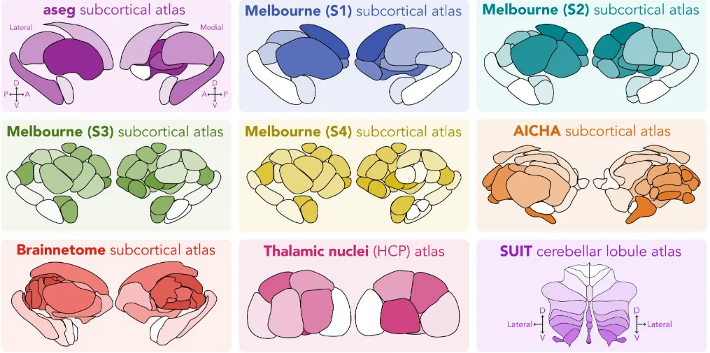
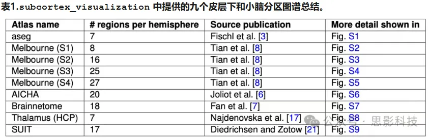
工具包涵盖的atlas不少：

我试了下我常用的Tian32 atlas（Melbourne S2)和红蓝配色，效果是这样的：

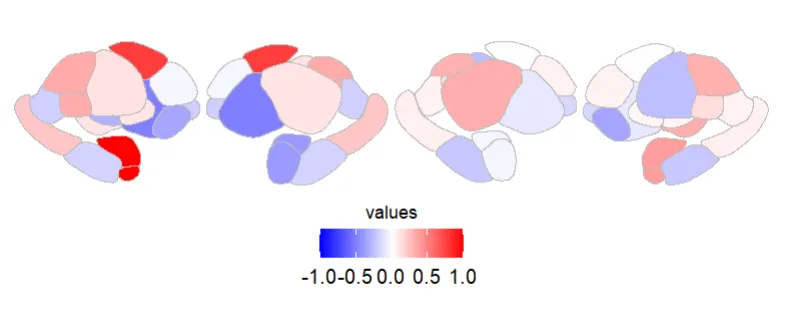
我在R里面是这么写的（示例）：

# plot on Tian_S2(Melbourne_S2) atlas, 32 subcortical ROIs

library(subcortexVisualizationR)

library(tidyverse)

# working dir

setwd(“D:/my_working_dir”)

# load my predefined color, a 256*3 matrix (blue-white-red)

my_colors <- read.csv(“my_color.csv”, header = FALSE)

color_strings <- rgb(my_colors[,1], my_colors[,2], my_colors[,3])

# load my data, a 1*32 vector 

# here generate random data and scale to [-1, 1]

set.seed(100)  

random_vector <- rnorm(32)  

abs_max <- max(abs(random_vector))

my_data <- random_vector / abs_max

# construct the data variable, right first, then left, according to your ROI order 

# the region name should follow your ROI order

# the region name should be identified by this package, so please refer to its extdata

# subcortexVisualizationR/inst/extdata/Melbourne_S2_L_ordering.csv

data_R <- data.frame(region = c(“hippocampus_anterior”, “hippocampus_posterior”, 

                                “amygdala_lateral”, “amygdala_medial”, 

                                “thalamus_DP”, “thalamus_VP”, 

                                “thalamus_VA”,”thalamus_DA”,

                                “accumbens_shell”,”accumbens_core”,

                                “pallidum_posterior”,”pallidum_anterior”,

                                “putamen_anterior”,”putamen_posterior”,

                                “caudate_anterior”,”caudate_posterior”),

                                 Hemisphere = ‘R’,

                                 value = my_data[1:16])

data_L <- data.frame(region = c(“hippocampus_anterior”, “hippocampus_posterior”, 

                                “amygdala_lateral”, “amygdala_medial”, 

                                “thalamus_DP”, “thalamus_VP”, 

                                “thalamus_VA”,”thalamus_DA”,

                                “accumbens_shell”,”accumbens_core”,

                                “pallidum_posterior”,”pallidum_anterior”,

                                “putamen_anterior”,”putamen_posterior”,

                                “caudate_anterior”,”caudate_posterior”),

                                 Hemisphere = ‘L’,

                                 value = my_data[17:32])

# combine data of two hemispheres

data_LR <- rbind(data_L, data_R)

# plot

plot_subcortical_data(subcortex_data=data_LR,

                      atlas = ‘Melbourne_S2′, hemisphere=’both’, 

                      line_color=’gray’, line_thickness=0.1,

                      cmap=color_strings,vmin=-1,vmax=1)

# save the picture

dev.print(png, file = file.path(data_dir,”my_pic.png”), 

          width = 2000, height = 1000, res = 300)