 夜雨聆风
夜雨聆风概述
核心定位
raster.py 是 GeoAI 的栅格数据处理核心工具集,本质是对 rasterio + GDAL 的工程封装,提供完整的栅格数据处理流水线。
功能架构
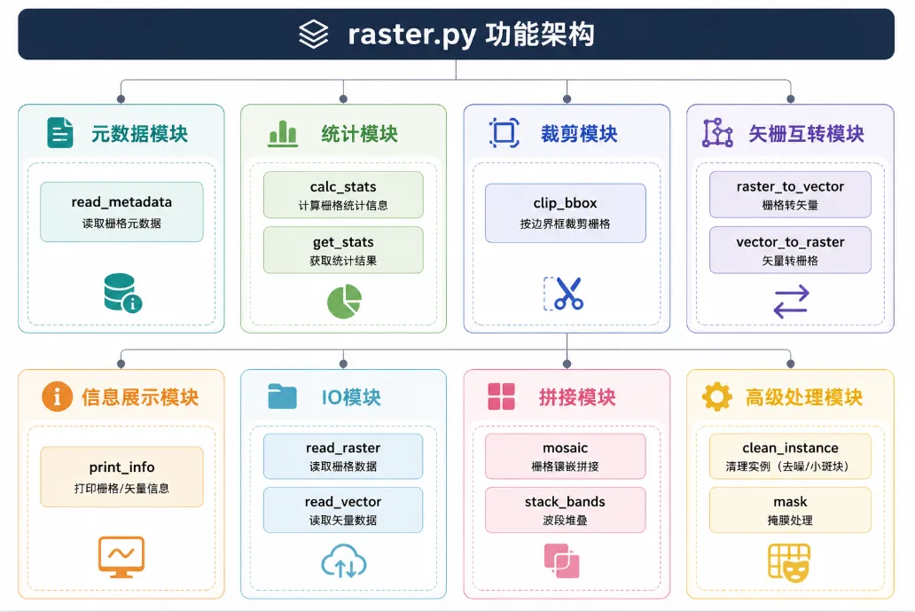
核心功能模块
模块分类总览
| 元数据 | read_raster_metadata | |
| 统计 | calc_statsget_raster_stats | |
| 信息展示 | get_raster_infoprint_raster_info | |
| 裁剪 | clip_raster_by_bbox | |
| 栅格→矢量 | raster_to_vectorraster_to_vector_batch | |
| 矢量→栅格 | vector_to_rasterbatch_vector_to_raster | |
| 拼接 | mosaic_geotiffs | |
| 波段堆叠 | stack_bands | |
| 高级处理 | clean_instance_mask | |
| IO | read_rasterread_vector |
关键函数详解
1. 元数据读取
read_raster_metadata
defread_raster_metadata(raster_path: str) -> RasterMetadata:""" 读取栅格元数据(不加载像素数据) 参数: raster_path: 栅格文件路径 返回: RasterMetadata 命名元组,包含: - crs: 坐标参考系统 - transform: 地理变换矩阵 - bounds: 地理边界 - width/height: 影像尺寸 - count: 波段数 - dtype: 数据类型 - nodata: 无数据值 - driver: 文件格式 """with rasterio.open(raster_path) as src:return RasterMetadata( crs=src.crs, transform=src.transform, bounds=src.bounds, width=src.width, height=src.height, count=src.count, dtype=src.dtypes[0], nodata=src.nodata, driver=src.driver, )设计要点:
• 使用 rasterio.open()但不读取像素,性能高效• 返回结构化的 NamedTuple,类型安全• 避免频繁打开文件造成的性能开销
2. 统计计算
calc_stats
defcalc_stats( image_files: List[str], max_samples: int = 1000, eps: float = 1e-6,) -> Tuple[np.ndarray, np.ndarray]:""" 计算数据集的 mean 和 std(近似统计) 参数: image_files: 影像文件列表 max_samples: 最大采样数(防止内存溢出) eps: 防止除零的小值 返回: (mean, std) 数组 """ n_channels = None total_sum = None total_sum_sq = None count = 0for f in image_files:with rasterio.open(f) as src:if n_channels isNone: n_channels = src.count total_sum = np.zeros(n_channels) total_sum_sq = np.zeros(n_channels)# 随机采样防止内存溢出 data = src.read() data = data.reshape((n_channels, -1)) samples = min(data.shape[1], max_samples // len(image_files))if samples > 0: idx = np.random.choice(data.shape[1], samples, replace=False) sampled = data[:, idx] total_sum += sampled.sum(axis=1) total_sum_sq += (sampled ** 2).sum(axis=1) count += samples mean = total_sum / count std = np.sqrt(total_sum_sq / count - mean ** 2 + eps)return mean, std设计要点:
• 随机采样策略:防止一次性加载大数据集导致内存溢出 • 近似统计:通过采样计算整体统计值,牺牲精度换取性能 • 数值稳定性:添加 eps防止标准差计算时除零
3. 栅格裁剪(重点)
clip_raster_by_bbox
defclip_raster_by_bbox( input_raster: str, output_raster: str, bbox: List[float], bands: Optional[List[int]] = None, bbox_type: str = "geo", # "geo" 或 "pixel" bbox_crs: Optional[str] = None,) -> str:""" 按边界框裁剪栅格 参数: input_raster: 输入栅格路径 output_raster: 输出栅格路径 bbox: 边界框坐标 bands: 要保留的波段列表(可选) bbox_type: 边界框类型(地理坐标/像素坐标) bbox_crs: 边界框的 CRS(跨 CRS 裁剪时使用) 返回: 输出栅格路径 """from rasterio.warp import transform_boundswith rasterio.open(input_raster) as src: src_crs = src.crsif bbox_type == "geo": minx, miny, maxx, maxy = bbox# 跨 CRS 坐标转换(关键)if bbox_crs isnotNoneand bbox_crs != src_crs: minx, miny, maxx, maxy = transform_bounds( bbox_crs, src_crs, minx, miny, maxx, maxy )# 生成裁剪窗口 window = src.window(minx, miny, maxx, maxy)else: # 像素坐标裁剪 min_row, min_col, max_row, max_col = bbox window = Window(min_col, min_row, max_col - min_col, max_row - min_row)# 读取并写出 data = src.read(window=window) if bands isNoneelse src.read(bands, window=window)with rasterio.open(output_raster, "w", **out_meta) as dst: dst.write(data)return output_raster核心流程:
bbox(地理/像素)→ 坐标转换(跨CRS)→ window → read(window) → write支持的裁剪模式:
geo | (minx, miny, maxx, maxy) | |
pixel | (min_row, min_col, max_row, max_col) |
4. 栅格→矢量(GeoAI核心)
raster_to_vector
defraster_to_vector( raster_path: str, output_path: Optional[str] = None, threshold: float = 0, min_area: float = 10, simplify_tolerance: Optional[float] = None, class_values: Optional[List[int]] = None, attribute_name: str = "class", output_format: str = "geojson",) -> gpd.GeoDataFrame:""" 将栅格标签转换为矢量多边形(polygonize) 参数: raster_path: 输入栅格路径 output_path: 输出矢量路径(可选) threshold: 二值化阈值 min_area: 最小多边形面积(过滤噪点) simplify_tolerance: 几何简化容差 class_values: 指定要矢量化的类别值列表 attribute_name: 属性字段名 output_format: 输出格式(geojson/shapefile/gpkg) 返回: GeoDataFrame 包含矢量化的多边形 """with rasterio.open(raster_path) as src: data = src.read(1) transform = src.transform crs = src.crs all_features = []if class_values isnotNone:# 按指定类别矢量化for class_val in class_values: mask = (data == class_val)for geom, value in features.shapes( mask.astype(np.uint8), mask=mask, transform=transform ): geom = shape(geom)if geom.area < min_area:continueif simplify_tolerance isnotNone: geom = geom.simplify(simplify_tolerance) all_features.append({"geometry": geom, attribute_name: class_val})else:# 全局矢量化 binary_mask = (data > threshold).astype(np.uint8)for geom, value in features.shapes( data.astype(np.int32), mask=binary_mask, transform=transform ): class_val = int(value)if class_val == 0:continue# ... 同样的过滤和简化处理 gdf = gpd.GeoDataFrame(all_features, crs=crs)if output_path isnotNone: gdf.to_file(output_path, driver="GeoJSON")return gdf核心API:features.shapes() - GDAL 的 polygonize 实现
关键处理步骤:
features.shapes() | ||
simplify() | ||
5. 矢量→栅格(训练标签核心)
vector_to_raster
defvector_to_raster( vector_path: Union[str, gpd.GeoDataFrame], output_path: Optional[str] = None, reference_raster: Optional[str] = None, attribute_field: Optional[str] = None, output_shape: Optional[Tuple[int, int]] = None, transform: Optional[Any] = None, pixel_size: Optional[float] = None, bounds: Optional[List[float]] = None, crs: Optional[str] = None,) -> np.ndarray:""" 将矢量数据转换为栅格(rasterize) 参数: vector_path: 输入矢量路径或 GeoDataFrame output_path: 输出栅格路径(可选) reference_raster: 参考栅格(自动继承尺寸和变换) attribute_field: 属性字段(用于像素值) output_shape: 输出尺寸(高, 宽) transform: 地理变换矩阵 pixel_size: 像素大小 bounds: 输出边界 crs: 坐标参考系统 返回: 栅格化后的 numpy 数组 """# 加载矢量数据 gdf = gpd.read_file(vector_path) ifisinstance(vector_path, str) else vector_path# 从参考栅格获取参数(最常用方式)if reference_raster isnotNone:with rasterio.open(reference_raster) as src: transform = src.transform output_shape = src.shape crs = src.crs# CRS对齐if gdf.crs != crs: gdf = gdf.to_crs(crs)# 构造 rasterize 输入 shapes = [(geom, value) for geom, value inzip(gdf.geometry, gdf[attribute_field])]# 栅格化 burned = features.rasterize( shapes=shapes, out_shape=output_shape, transform=transform, fill=0, dtype=np.uint8, )if output_path isnotNone:with rasterio.open(output_path, "w", **metadata) as dst: dst.write(burned, 1)return burned三种输入方式:
reference_raster | ||
transform + output_shape | ||
bounds + pixel_size |
核心API:features.rasterize() - GDAL 的 rasterize 实现
6. 影像拼接
mosaic_geotiffs
defmosaic_geotiffs( input_files: List[str], output_path: str, crs: Optional[str] = None, resolution: Optional[Tuple[float, float]] = None, nodata: Optional[float] = None,) -> str:""" 将多个 GeoTIFF 文件拼接为一个文件 参数: input_files: 输入文件列表 output_path: 输出文件路径 crs: 输出 CRS(可选) resolution: 输出分辨率(可选) nodata: 无数据值(可选) 返回: 输出文件路径 """# 使用 GDAL 构建 VRT vrt_path = "temp.vrt" gdal.BuildVRT(vrt_path, input_files)# 转换为 GeoTIFF gdal.Translate(output_path, vrt_path, format="GTiff", creationOptions=["COMPRESS=DEFLATE"])# 可选:构建金字塔with rasterio.open(output_path, "r+") as dst: dst.build_overviews([2, 4, 8, 16])return output_path核心流程:
多个 GeoTIFF → VRT(虚拟栅格)→ Translate → 金字塔 → COG7. 波段堆叠
stack_bands
defstack_bands( input_files: List[str], output_file: str, resolution: Optional[float] = None, dtype: Optional[str] = None,) -> str:""" 将多个单波段影像堆叠为多波段影像 参数: input_files: 输入文件列表(按波段顺序) output_file: 输出文件路径 resolution: 输出分辨率 dtype: 输出数据类型 返回: 输出文件路径 """# 构建 VRT vrt_cmd = ["gdalbuildvrt", "-separate", "stack.vrt"] + input_files subprocess.run(vrt_cmd, check=True)# 转换为多波段 GeoTIFF translate_cmd = ["gdal_translate","-tr", str(resolution), str(resolution),"stack.vrt", output_file,"-of", "COG", ] subprocess.run(translate_cmd, check=True)return output_file8. 实例分割结果优化
clean_instance_mask
defclean_instance_mask( input_path: str, output_path: Optional[str] = None, min_area: int = 50, fill_holes: bool = True, max_hole_area: int = 100, smooth: bool = True, smooth_sigma: float = 1.5,) -> str:""" 清理实例分割掩码(保留实例身份) 参数: input_path: 输入掩码路径 output_path: 输出路径(可选) min_area: 最小实例面积 fill_holes: 是否填充孔洞 max_hole_area: 最大填充孔洞面积 smooth: 是否平滑边界 smooth_sigma: 高斯平滑参数 返回: 输出路径 """with rasterio.open(input_path) as src: mask = src.read(1)# 1. 删除小实例 labeled, num_labels = measure.label(mask, connectivity=2, return_num=True) props = measure.regionprops(labeled)for prop in props:if prop.area < min_area: mask[labeled == prop.label] = 0# 2. 填充孔洞if fill_holes: holes = mask == 0 labeled_holes, _ = ndi.label(holes)for prop in measure.regionprops(labeled_holes):if prop.area < max_hole_area: coords = prop.coords# 填充为周围区域的值 ...# 3. 平滑边界if smooth: mask = gaussian_filter(mask.astype(float), sigma=smooth_sigma)if output_path isnotNone:with rasterio.open(output_path, "w", **meta) as dst: dst.write(mask.astype(np.uint8), 1)return output_path处理步骤:
使用示例
示例 1:元数据读取
import geoai# 读取元数据(不加载像素)metadata = geoai.read_raster_metadata("satellite.tif")print(f"影像尺寸: {metadata.width} x {metadata.height}")print(f"波段数: {metadata.count}")print(f"坐标系统: {metadata.crs}")print(f"数据类型: {metadata.dtype}")print(f"地理边界: {metadata.bounds}")示例 2:统计计算
import geoaiimport glob# 获取数据集统计image_files = glob.glob("dataset/*.tif")mean, std = geoai.calc_stats(image_files)print(f"Mean: {mean}")print(f"Std: {std}")# 单影像统计stats = geoai.get_raster_stats("image.tif")print(f"波段1 均值: {stats['mean'][0]:.2f}")print(f"波段1 标准差: {stats['std'][0]:.2f}")示例 3:栅格裁剪
import geoai# 方式1:地理坐标裁剪geoai.clip_raster_by_bbox( input_raster="input.tif", output_raster="clipped_geo.tif", bbox=[116.0, 39.0, 116.5, 39.5], # (minx, miny, maxx, maxy) bbox_type="geo", bbox_crs="EPSG:4326", # WGS84 bands=[1, 2, 3] # 只保留 RGB 波段)# 方式2:像素坐标裁剪geoai.clip_raster_by_bbox( input_raster="input.tif", output_raster="clipped_pixel.tif", bbox=[0, 0, 512, 512], # (min_row, min_col, max_row, max_col) bbox_type="pixel")示例 4:栅格→矢量
import geoai# 将分类结果矢量化gdf = geoai.raster_to_vector( raster_path="classification.tif", output_path="polygons.geojson", threshold=0.5, # 二值化阈值 min_area=100, # 最小面积过滤 simplify_tolerance=2.0, # 几何简化 class_values=[1, 2, 3] # 只矢量化类别1、2、3)print(f"生成了 {len(gdf)} 个多边形")示例 5:矢量→栅格
import geoai# 方式1:使用参考栅格(最常用)geoai.vector_to_raster( vector_path="buildings.geojson", output_path="buildings_mask.tif", reference_raster="satellite.tif", # 自动对齐 attribute_field="class"# 使用 class 字段作为像素值)# 方式2:手动指定参数geoai.vector_to_raster( vector_path="roads.geojson", output_path="roads_mask.tif", output_shape=(1000, 1000), transform=src.transform, crs="EPSG:32650", attribute_field="road_type")示例 6:影像拼接
import geoaiimport glob# 拼接多个影像input_files = glob.glob("tiles/*.tif")geoai.mosaic_geotiffs( input_files=input_files, output_path="mosaic.tif", crs="EPSG:32650", resolution=(1.0, 1.0))print("拼接完成!")示例 7:波段堆叠
import geoai# 将单波段影像堆叠为多波段geoai.stack_bands( input_files=["band1.tif", "band2.tif", "band3.tif", "band4.tif"], output_file="stacked.tif", resolution=1.0, dtype="UInt16")print("波段堆叠完成!")示例 8:实例分割结果优化
import geoai# 清理实例分割掩码geoai.clean_instance_mask( input_path="instance_mask.tif", output_path="cleaned_mask.tif", min_area=50, # 最小实例面积 fill_holes=True, # 填充孔洞 max_hole_area=100, # 最大孔洞面积 smooth=True, # 平滑边界 smooth_sigma=1.5# 平滑参数)print("实例掩码清理完成!")工程架构总结
核心技术栈
GeoAI raster 模块 = rasterio(栅格读写/窗口操作) + GDAL(拼接/格式转换/COG) + numpy(数组处理) + geopandas(矢量处理) + scipy(图像处理)设计特点
| 工程级封装 | |
| 内存优化 | |
| 类型安全 | |
| 自动对齐 | |
| 多格式支持 |
典型工作流
1. 数据准备 └── download → clip → mosaic → stack_bands2. 训练数据生成 └── vector_to_raster(标签栅格化)3. 推理后处理 └── raster_to_vector(结果矢量化)→ clean_instance_mask(优化)4. 数据分析 └── read_raster_metadata → calc_stats → visualize