 夜雨聆风
夜雨聆风


R包神器 | ape (九) 基本和高级功能 – 几何及复合图形,自建函数

6 几何及复合图形
6.1 单绘图区
现在,我们可以在绘制树图时看到图形的一些几何细节。我们首先设置外边距 (Outer margins, 图形参数oma),默认为0,然后通过调用box() 3次并使用适当的选项来显示内、外边距:
# oma: 预设外边距的宽度par(oma = rep(2, 4))# [1] 2 2 2 2plot(mytr)# 从内到外4个区域:"plot"(默认), "figure", "inner" and "outer"box(lty = 3) # lty - 设置线条样式(Line type),可取0、1、2、3、4、5、6,分别表示:不划线;实线;虚线;点线;点划线;长划线;点长划线box("figure", col = "blue")# mtext: 将文本写至图形的边距(Margins)# 顺序(顺时针):下、左、上、右# 预设的外边距宽度不足时,影响此文本的展示for (i in 1:4)mtext("Outer margin", i, 0.5, outer = TRUE, font = 2, col = "blue")box("outer") # 在整个绘图区的最外层画框for (i in 1:4)mtext("Inner margin", i, 0.5, outer = FALSE, font = 2, col = "brown")
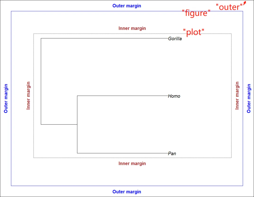
1. par()的oma选项: 预设外边距的宽度(默认无外边距);2. 从内到外4个区域:”plot”(默认), “figure”, “inner” and “outer”;3. mtext(): 将文本写至图形的边距(Margins),顺序(顺时针):下、左、上、右,预设的外边距宽度不足时,影响此文本的展示。
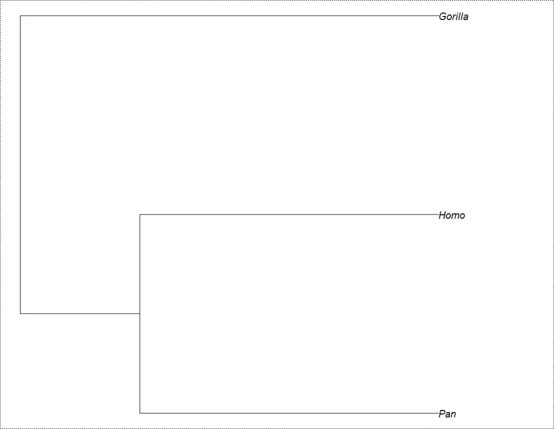
当然,也可以使用par(mar = ….)更改内边距。请注意,在运行plot(mytr)之前,进行plot(mytr, no.margin = TRUE)与调用parpar(mar = rep(0, 4))是相同的。
plot(mytr, no.margin = TRUE)box("plot", lty = 3)
6.2 多重布局 (Multiple Layout)
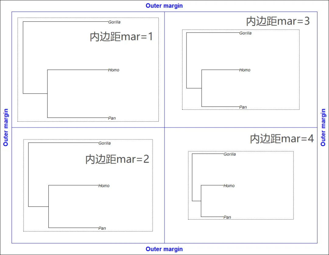
通过先使用layout函数拆分图形设备,可在同一图形上绘制多棵树。在这种情况下,每个图形都有自己的1组内边距 (可与下个示例中的不同),但外边距是图形的”全局“(Global)边距:
matrix(1:4, 2, 2)# [,1] [,2]# [1,] 1 3# [2,] 2 4layout(matrix(1:4, 2, 2))par(oma = rep(2, 4))for (i in 1:4) {par(mar = rep(i, 4))plot(mytr)box(lty = 3)box("figure", col = "blue")}for (i in 1:4)mtext("Outer margin", i, 0.5, outer = TRUE, font = 2, col = "blue")box("outer")
分割图形设备的另1种方法是调用par(mfcol = c(2, 2))。但是,建议使用更灵活、强大的layout函数:
· layout具有width和height选项,提供图形的行和列的(相对)大小。
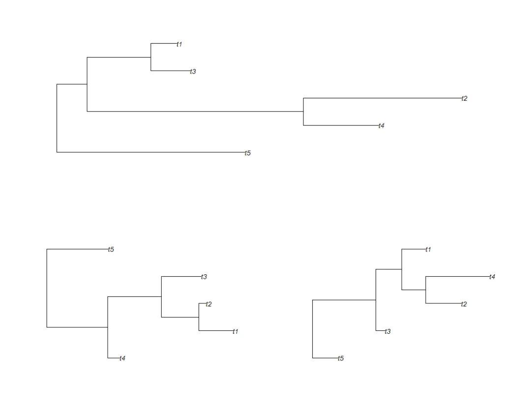
· 作为layout的主要参数的矩阵是图形布局的符号表示:单个图形可跨越矩阵的多个单元;例如,layout(matrix(c(1, 2, 1, 3), 2, 2))将在设备上指定3个绘图,第1个绘图跨越第一行,第2行拆分为2个绘图:
layout(matrix(c(1, 2, 1, 3), 2, 2))for (i in 1:3) plot(rtree(5))
7 构建自己的代码和函数
在本节中,我们将研究利用ape的图形功能来构建代码或函数的2种方法。
7.1 获取已录入的参数
每次调用plot.phylo时,一些数据和参数都保存在特定的R环境(R的一组对象所占用的计算机内存的一部分)中,然后由nodelabels等函数使用。此环境称为.PlotPhyloEnv,可供所有用户访问,因此可通过以下方式获取列表(List) last_plot.phylo:
(pp <- get("last_plot.phylo", envir = .PlotPhyloEnv))# $type# [1] "phylogram"# $use.edge.length# [1] TRUE# $node.pos# [1] 1# $node.depth# [1] 1# $show.tip.label# [1] TRUE# $show.node.label# [1] FALSE# $font# [1] 3# $cex# [1] 0.83# $adj# [1] 0# $srt# [1] 0# $no.margin# [1] FALSE# $label.offset# [1] 0# $x.lim# [1] 0.000000 2.565094# $y.lim# [1] 1 5# $direction# [1] "rightwards"# $tip.color# [1] "black"# $Ntip# [1] 5# $Nnode# [1] 4# $root.time# NULL# $align.tip.label# [1] FALSE# $edge# [,1] [,2]# [1,] 6 1# [2,] 6 7# [3,] 7 2# [4,] 7 8# [5,] 8 9# [6,] 9 3# [7,] 9 4# [8,] 8 5# $xx# [1] 0.3416120 0.9779764 1.9980659 2.3773992 1.5240125 0.0000000 0.8540463 1.2019900 1.5262024# $yy# [1] 1.0000 2.0000 3.0000 4.0000 5.0000 2.0625 3.1250 4.2500 3.5000
大多数记录的参数对应于plot.phylo的参数。该列表中存储的最后2个向量xx和yy是树的尖端和节点(Tip+Node 逆时针顺序?)的坐标。
7.2 布局覆盖 (Overlaying Layouts)
graphics包无法轻松地与多重布局(Multiple layout)上的图形交互。例如,在调用layout并完成第2个绘图之后,就无法向第1个图形添加元素 (点、箭头等),这限制了以图形方式连接这些绘图的可能性。但是,命令par(new = TRUE)提供了1种方法,如这里所述。
其思想是跟踪整个图形设备上节点 (及其它图形元素 (如果需要)) 的坐标。但是,由于图形/plots很可能使用不同的坐标系 (例如,由于分枝长度的比例不同),因此必须将这些坐标转换为图形/graphical设备上的物理单位 (通常为英寸)。由于par()在许多参数中返回绘图区域/Plotting region、边距/Margins和设备的物理尺寸(英寸),并分别使用参数“pin”、“mai”和“din” (figure大小也有“fin”,其不包括外边距,如果这些外部边距不为0,则需要使用)。我们将在这里使用的另1个图形参数由par(“usr”)给出,给出绘图区域坐标的极值。
步骤如下:
1. 重新缩放(Rescale)每个树形图的节点坐标,使其介于0和1之间。
2. 通过将这些坐标与“fin”中的相关值相乘,并添加相关边距的大小(英寸),以英寸为单位转换这些坐标。这将给出每个图形/Figure(即,包括边距)中以英寸为单位的坐标。
3. 使用layout最终定义的几何图形添加到上一步输出的坐标中。
完成这3个步骤后,我们将获得整个设备上节点的坐标,单位为英寸,与每个绘图/Plot中使用的各种标尺(Scales)无关。然后,对par(new = TRUE)的调用使得没有绘制任何内容,并且R不会删除设备上已经绘制的内容。然后,我们调用plot(NA),选项为type = “n”、ann = FALSE、axes = FALSE,从而生成一个“裸/Bare”图。这里的重要选项是[x|y]lim = 0:1,用于设置每个轴上的比例尺(Scale),以及[x|y]axs = “i”,用于设置轴(Axes)以精确扩展到数据的范围或指定的限制(Limits) (默认情况下,xaxs和yaxs等于“r”,这将在数据范围或限制的两边各添加4%)。
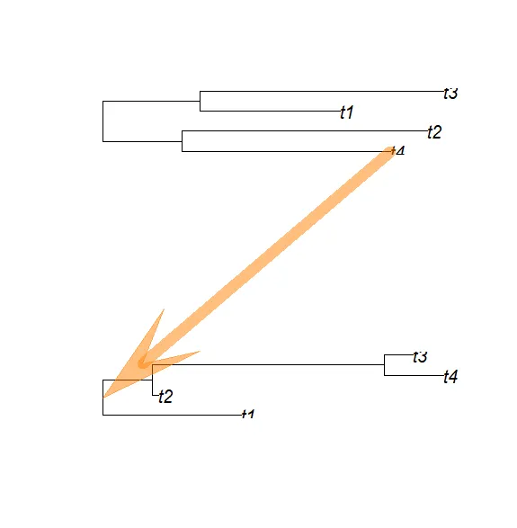
然而,在类似于本(代码.R)文档的小实例(Vignette)中,每次调用plot都会打开一个新设备(Device),因此无法交互地执行上述步骤。相反,下一组命令包含一些注释并打印一些中间结果。在此示例中,将绘制两棵随机树,并用箭头将第1棵树的第1个尖端连接到第2棵树的根:
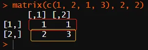
matrix(1:2, 2)# [,1]# [1,] 1# [2,] 2## split the device into 2:layout(matrix(1:2, 2))## plot the 1st treeplot(rtree(4))## get the parameters of this first plot:pp <- get("last_plot.phylo", envir = .PlotPhyloEnv)## keep the coordinates of the first tip:x <- pp$xx[1]y <- pp$yy[1]## extremes of the coordinates on both axes:(pu <- par("usr"))# [1] -0.04985097 1.29612512 0.88000000 4.12000000## fraction of the plot region:(x - pu[1]) / (pu[2] - pu[1])# [1] 0.78789(y - pu[3]) / (pu[4] - pu[3])# [1] 0.03703704## get the dimensions of plotting region and margins in inches:pi <- par("pin")mi <- par("mai")## convert the coordinates into inches:xi1 <- (x - pu[1]) / (pu[2] - pu[1]) * pi[1] + mi[2]yi1 <- (y - pu[3]) / (pu[4] - pu[3]) * pi[2] + mi[1]## xi1 and yi1 are the final coordinates of this tip in inches## plot the 2nd tree:plot(rtree(4))## same as above:pp <- get("last_plot.phylo", envir = .PlotPhyloEnv)## ... except we take the coordinates of the root:x <- pp$xx[5]y <- pp$yy[5]pu <- par("usr")pi <- par("pin")mi <- par("mai")xi2 <- (x - pu[1]) / (pu[2] - pu[1]) * pi[1] + mi[2]yi2 <- (y - pu[3]) / (pu[4] - pu[3]) * pi[2] + mi[1]## xi2 and yi2 are the final coordinates of this root in inches## we add the height of this second plot to the 'y' coordinate## of the first tip of the first tree which is above the second## one according to layout()yi1 <- yi1 + par("fin")[2]## => this operation depends on the specific layout of plots## get the dimension of the device in inches:di <- par("din")## reset the layoutlayout(1)## set new = TRUE and the margins to zero:par(new = TRUE, mai = rep(0, 4))## set the scales to be [0,1] on both axes (in user coordinates):plot(NA, type = "n", ann = FALSE, axes = FALSE, xlim = 0:1,ylim = 0:1, xaxs = "i", yaxs = "i")## graphical elements can now be added:fancyarrows(xi1/di[1], yi1/di[2], xi2/di[1], yi2/di[2], 1,lwd = 10, col = rgb(1, .5, 0, .5), type = "h")
此代码必须适应于精确的布局,以便在x-或y-方向上适当移动坐标。下一个bloc定义了1个函数,该函数使用上述代码绘制2个树,并从第1棵树的参数from指定的尖端,向第2棵树的根添加箭头:
foo <- function(phy1, phy2, from){layout(matrix(1:2, 2))plot(phy1, font = 1)pp <- get("last_plot.phylo", envir = .PlotPhyloEnv)from <- which(phy1$tip.label == from)x <- pp$xx[from]y <- pp$yy[from]## fraction of the plot region:pu <- par("usr")## convert into inches:pi <- par("pin")mi <- par("mai")xi1 <- (x - pu[1]) / (pu[2] - pu[1]) * pi[1] + mi[2]yi1 <- (y - pu[3]) / (pu[4] - pu[3]) * pi[2] + mi[1]plot(phy2)pp <- get("last_plot.phylo", envir = .PlotPhyloEnv)to <- Ntip(phy2) + 1x <- pp$xx[to]y <- pp$yy[to]## same as above:pu <- par("usr")pi <- par("pin")mi <- par("mai")xi2 <- (x - pu[1]) / (pu[2] - pu[1]) * pi[1] + mi[2]yi2 <- (y - pu[3]) / (pu[4] - pu[3]) * pi[2] + mi[1]yi1 <- yi1 + par("fin")[2]di <- par("din")layout(1)par(new = TRUE, mai = rep(0, 4))plot(NA, type = "n", ann = FALSE, axes = FALSE, xlim = 0:1,ylim = 0:1, xaxs = "i", yaxs = "i")fancyarrows(xi1/di[1], yi1/di[2], xi2/di[1], yi2/di[2], 1,lwd = 10, col = rgb(1, .5, 0, .5), type = "h")}
我们用哺乳动物目进化树尝试此功能,我们希望将其与我们的小树mytr连接:
trb <- read.tree(text = "((Primates,Carnivora),Monotremata);")par(xpd = TRUE)foo(trb, mytr, "Carnivora")# foo(trb, mytr, "Primates")
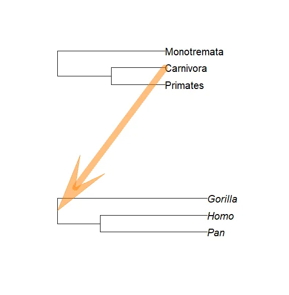
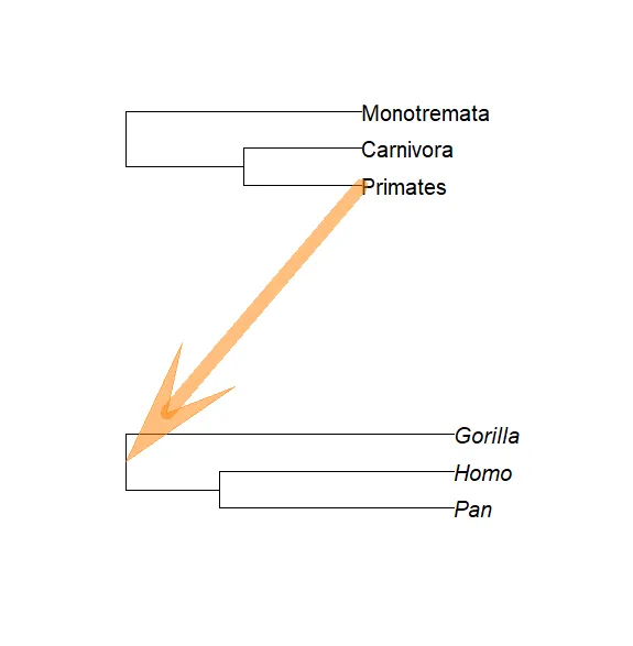
请注意,第1棵树没有分枝长度,因此两棵树的比例尺(Scales)明显不同。
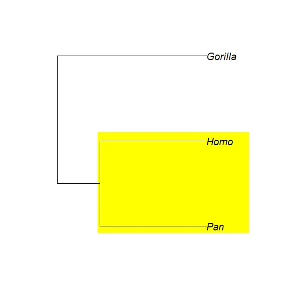
这些功能的另1个用途是绘制着色矩形(Coloured rectangles)背景来划分分枝。同样,我们可以使用par(new = TRUE)和plot.phylo的plot=FALSE选项,该选项打开并设置图形设备,坐标取自第2.2节详述的树,但未绘制任何图形。然后,用户可以调用任何低级绘图命令,然后在par(new = TRUE)之后使用plot()。例如,如果我们想画1个矩形来显示由人类和黑猩猩组成的分枝:
plot(mytr, plot = FALSE)# 继承自 已经绘制的图形(即使不可见) 的内部元素的性质:pp <- get("last_plot.phylo", envir = .PlotPhyloEnv)# 选取tip+node的坐标(逆时针),定义矩形的4个边(左、下、右、上):rect(pp$xx[5] - 0.1, pp$yy[1] - 0.1, pp$xx[1] + 2, pp$yy[2] + 0.1,col = "yellow", border = NA)par(new = TRUE)plot(mytr)
有几种方法可以找到矩形的限制/Limits:根据经验尝试不同的值;在具有进化树的第1个草图上使用locator();或者使用类似于上一个示例的计算。?phydataplot中的例子给出了使用par(new = TRUE)的其它示例。
References
[3] P. Murrell. R Graphics. Chapman & Hall/CRC, Boca Raton, FL, 2006.
完
通过过去几篇文章对ape这个进化树领域的经典R包的了解,系统地熟悉了相关数据分析与绘图的概念、术语等,如:Tip、Node、Edge,phylogram、cladogram,coalescent … … 推测这些概念在不同的工具中大体通用,因此准确地把握这些概念非常重要。
后续将使用ape进行贝叶斯天际线图等图形的制作,继续深入学习进化树分析与可视化相关的原理和技术。