AI工具|Positron中使用Claude Code(接入国产大模型)

❝

过去两年，AI工具的迭代速度几乎超出了所有人的预期。从最初的文本生成，到如今能够辅助数据分析、代码编写、文献检索，乃至参与复杂的科学推理。

AI正在以我们从未见过的方式，悄然改变各个专业领域的工作方式。但个人认为，AI不是来替代我们判断力的，而是在那些耗时耗力的环节，帮我们腾出更多精力，专注于真正需要专业思考的地方。

本次介绍Positron + Claude Code + 国产大模型。这个组合为我们提供了一条相对顺畅的AI辅助编程路径。不需要解决复杂的网络问题，也不需要高昂的API成本，就能在日常工作中引入AI协作。

AI在变，我们也需跟着变。不是盲目追风，而是保持开放，主动探索，让AI工具真正为我们所用。

❞

Positron软件

「Positron」 是由Posit公司（即原 RStudio 公司，2022年更名）开发的新一代数据科学IDE，目前仍处于Public Beta阶段。它基于VS Code的开源内核（code-server） 构建，本质上是一个深度定制的 VS Code。Positron是 Posit对RStudio 的”接班人”规划，但两者目前并行存在，定位不同，具体如下：

「如果你主要用 R 做分析，RStudio 依然够用且更稳定。但如果你同时涉及 Python、需要丰富的 VS Code 插件生态（比如 Claude Code），Positron 是值得尝试的选择」

Claude code

「Claude Code」 是Anthropic推出的AI编程助手，是一个能理解整个项目、主动读写文件、执行命令的AI代理（Agent）。核心能力在于它能感知上下文——它不只是看你问的那一句话，而是会主动去读你的项目文件、了解你的代码结构，再给出有针对性的回答。这一点是普通聊天式 AI做不到的。打个比方：普通AI插件像一个坐在旁边回答问题的助手，而Claude Code更像一个能直接上手帮你干活的同事——它能看懂你的项目结构，知道你在做什么，然后直接动手修改代码、跑脚本、查错误。

• 四种使用方式：

本文将介绍「Positron插件」的使用方式。

同时Claude Code本身只是一个壳——一个能读文件、执行命令、管理对话的工具框架。它本身不包含任何 AI 能力，所有的”智能”都来自背后调用的「大语言模型」。Claude Code可以连接Anthropic自家的Claude模型（如 Claude Sonnet、Claude Opus）。但Claude模型未对中国开放，使用该模型需要解决网络问题，而且模型收费也较贵。一种替代方案是使用「国产模型」。因为Claude Code 支持自定义API地址，只要国内模型提供兼容OpenAI格式的API接口，就可以直接替换。目前主流国产模型均已支持，比如DeepSeek、GLM、Kimi、Qwen等。

国产大语言模型

下面是由Gemini生成的一个国产大语言模型对比图：

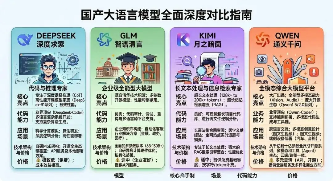
本文将介绍如何接入「DeepSeek」。

Positron中使用Claude code

本文将介绍「Positron插件Claude Code+国产大语言模型DeepSeek」

「STEP 1」：安装Positron

直接搜索Positron官网：https://positron.posit.co/ ，进入之后点击「Free Download」，之后按照正常的软件安装流程即可。

「STEP 2」：安装Claude Code插件

完成STEP 1之后，打开Positron，找到图中所示①「Extensions」，搜索Claude Code。选择图中所示②「Claude Code for VS Code」，点击「Install」

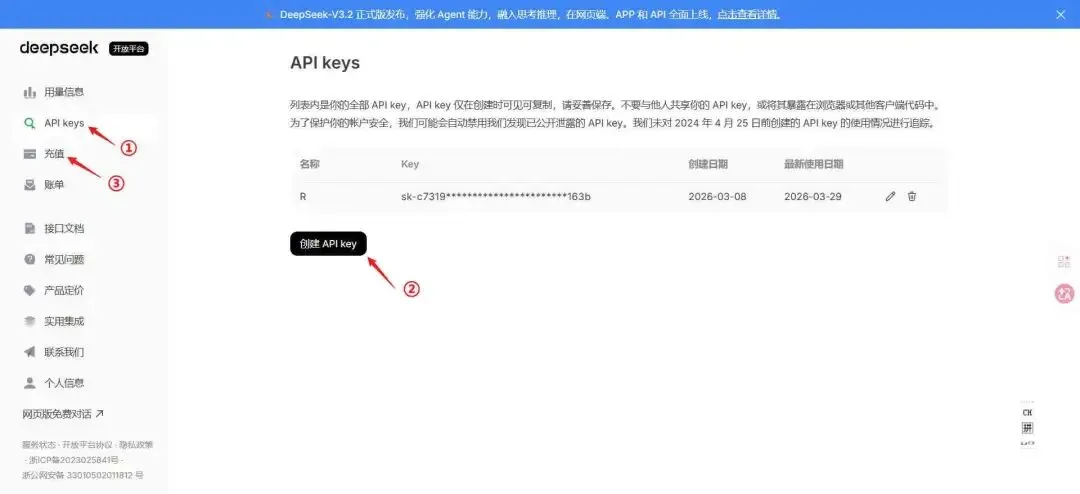
「STEP 3」：接入国产大模型(DeepSeek)配置

完成STEP2之后，进行模型配置，具体步骤详见下图：

打开setting.json文件后，将下面这段复制上去。「API-key」换成真实的API。

{"name":"ANTHROPIC_BASE_URL", "value":"https://api.deepseek.com/anthropic" }, {"name":"ANTHROPIC_AUTH_TOKEN", "value":"API-key" }, {"name":"API_TIMEOUT_MS", "value":600000 }, {"name":"ANTHROPIC_MODEL", "value":"deepseek-chat" }, {"name":"ANTHROPIC_SMALL_FAST_MODEL", "value":"deepseek-chat" }, {"name":"CLAUDE_CODE_DISABLE_NONESSENTIAL_TRAFFIC", "value":1 },

真实的API获取，可以直接搜索「DeepSeek 开放平台」https://platform.deepseek.com/usage 。可以先充值10元体验一下。

「STEP 4」：可使用Claude Code AI辅助编程

STEP 1~STEP 3完成之后，我们就可以体验一下。

下图为一个示例，我之前文件test.R是空文件，仅用一句话，自动生成所有代码在test.R文件中。

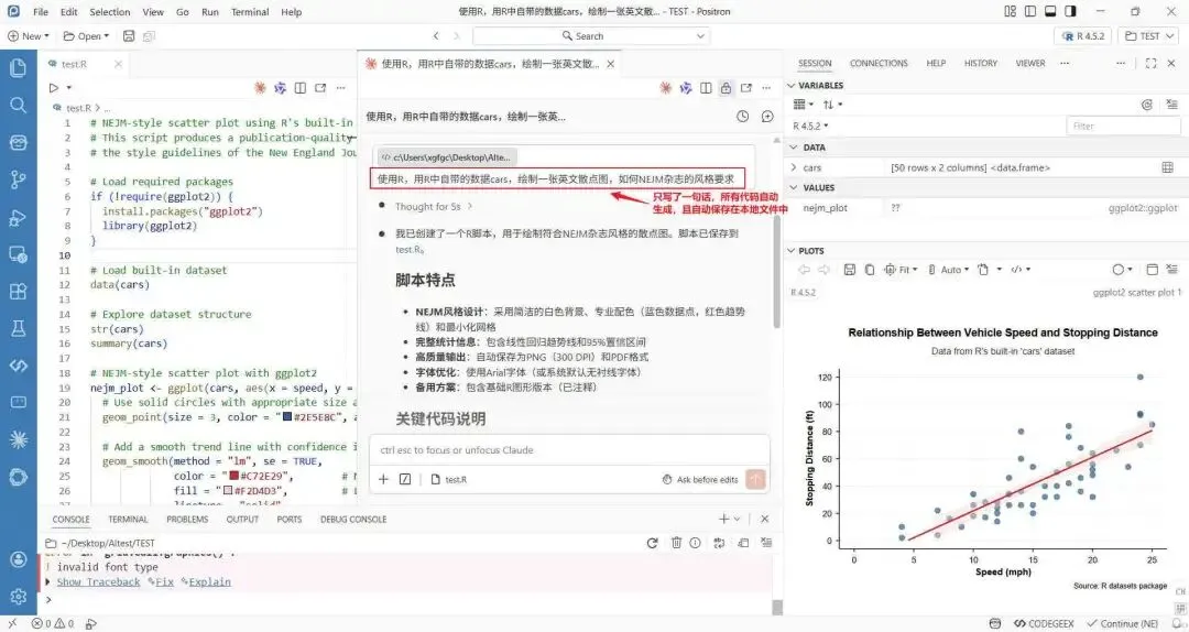
Claude Code自动生成的代码：

# NEJM-style scatter plot using R's built-in cars dataset# This script produces a publication-quality scatter plot following# the style guidelines of the New England Journal of Medicine (NEJM)# Load required packagesif (!require(ggplot2)) {  install.packages("ggplot2")library(ggplot2)}# Load built-in datasetdata(cars)# Explore dataset structurestr(cars)summary(cars)# NEJM-style scatter plot with ggplot2nejm_plot <- ggplot(cars, aes(x = speed, y = dist)) +# Use solid circles with appropriate size and color  geom_point(size = 3, color = "#2E5E8C", alpha = 0.7) +  # NEJM-like blue# Add a smooth trend line with confidence interval  geom_smooth(method = "lm", se = TRUE,              color = "#C72E29",        # NEJM-like red for trend line              fill = "#F2D4D3",         # Light red for confidence band              linetype = "solid",              size = 1) +# Customize theme for NEJM style  theme_minimal(base_size = 12) +  theme(# Clean, minimal background    panel.background = element_rect(fill = "white", color = NA),    plot.background = element_rect(fill = "white", color = NA),# Axis lines and ticks    axis.line = element_line(color = "black", size = 0.5),    axis.ticks = element_line(color = "black", size = 0.5),    axis.ticks.length = unit(0.15, "cm"),# Axis text    axis.text = element_text(color = "black", size = 11, family = "Arial"),    axis.title = element_text(color = "black", size = 12, face = "bold",                              family = "Arial", margin = margin(t = 10, r = 10)),# Plot title and subtitle    plot.title = element_text(size = 14, face = "bold", hjust = 0.5,                              family = "Arial", margin = margin(b = 10)),    plot.subtitle = element_text(size = 12, hjust = 0.5, color = "#333333",                                 family = "Arial", margin = margin(b = 15)),# Grid lines (minimal or none)    panel.grid.major = element_line(color = "#F0F0F0", size = 0.3),    panel.grid.minor = element_blank(),# Plot margins    plot.margin = unit(c(1, 1, 1, 1), "cm")  ) +# Labels and titles  labs(    title = "Relationship Between Vehicle Speed and Stopping Distance",    subtitle = "Data from R's built-in 'cars' dataset",    x = "Speed (mph)",    y = "Stopping Distance (ft)",    caption = "Source: R datasets package"  ) +# Axis limits and breaks  scale_x_continuous(breaks = seq(0, 25, by = 5), limits = c(0, 25)) +  scale_y_continuous(breaks = seq(0, 120, by = 20), limits = c(0, 120))# Display the plotprint(nejm_plot)# Save the plot in high resolutionggsave("nejm_scatterplot.png",       plot = nejm_plot,       width = 8,       height = 6,       dpi = 300,       bg = "white")ggsave("nejm_scatterplot.pdf",       plot = nejm_plot,       width = 8,       height = 6,       bg = "white")# Alternative: Base R version for minimal dependency# Uncomment to use base R graphics# pdf("nejm_scatterplot_base.pdf", width = 8, height = 6)# par(mar = c(5, 5, 4, 2) + 0.1,  # Margins#     family = "sans",            # Sans-serif font#     cex.axis = 1.1,             # Axis text size#     cex.lab = 1.2,              # Axis label size#     font.lab = 2,               # Bold axis labels#     bty = "l",                  # L-shaped box#     tcl = -0.3)                 # Tick length## plot(cars$speed, cars$dist,#      pch = 19,                  # Solid circles#      col = "#2E5E8C",           # NEJM-like blue#      cex = 1.5,                 # Point size#      xlab = "Speed (mph)",#      ylab = "Stopping Distance (ft)",#      main = "Relationship Between Vehicle Speed and Stopping Distance",#      xlim = c(0, 25),#      ylim = c(0, 120),#      axes = FALSE)              # Custom axes## # Add custom axes# axis(1, at = seq(0, 25, 5), lwd = 1, lwd.ticks = 1)# axis(2, at = seq(0, 120, 20), lwd = 1, lwd.ticks = 1, las = 1)## # Add grid# grid(nx = NA, ny = NULL, lty = 2, col = "gray90")## # Add regression line# abline(lm(dist ~ speed, data = cars),#        col = "#C72E29", lwd = 2)## # Add confidence interval# conf_int <- predict(lm(dist ~ speed, data = cars),#                     interval = "confidence")# lines(cars$speed, conf_int[, "lwr"], col = "#C72E29", lty = 2)# lines(cars$speed, conf_int[, "upr"], col = "#C72E29", lty = 2)## dev.off()

「Positron插件待改进的地方」：无法识别上传的图标。